
Solving Latin Squares as Constraint Satisfaction Problems using Backtracking Search with Heuristics
A Latin square is an n x n grid filled with n different symbols (commonly numbers 1 to n), each appearing exactly once in every row and every column.
An example of a 3x3 Latin square would look like the following table:
| 1 | 2 | 3 |
|---|---|---|
| 3 | 1 | 2 |
| 2 | 3 | 1 |
In this post, I will illustrate the key concepts of constraint satisfaction problems (CSPs) and backtracking search, two fundamental techniques in AI, by applying them to solve Latin squares.
Constraint Satisfaction
Constraint satisfaction is a subfield of optimization that focuses on selecting the best option from a set of possible options. It ensures that a solution meets all given constraints, such as resource limitations or time restrictions. Once these constraints are met, the next goal is to optimize a given function, either by maximizing or minimizing it.
In a constraint satisfaction problem (often abbreviated as CSP), variables must be assigned values while meeting specific conditions.
For a computer to solve this problem, the problem must be clearly structured. The key properties of a CSP are:
- Variables: The set of possible values that each variable can take.
- Domains: The possible values (options) for a variable.
- Constraints: The specific conditions that must be satisfied when assigning values to the variables.
The constraints in particular can be categorized based on how many variables they involve:
- Unary Constraint: A constraint that involves only one variable, restricting the values it can take from its domain.
- Binary Constraint: A constraint that involves two variables, specifying the allowable pairs of values between them.
One of the most well-known examples of a CSP is Sudoku. In the context of Sudoku, the properties can be described as follows:
- Variables: The empty squares on the Sudoku grid.
- Domains: The set
{1, 2, 3, 4, 5, 6, 7, 8, 9}, representing the possible digits for each empty square. - Constraints: No digit can repeat in any row, column, or 3x3 subgrid.
In the context of a 3x3 Latin square, each property of CSP can be described as follows:
-
Variables:
{(0, 0), (0, 1), (1, 1), (1, 0), (1, 1), (1, 2), (2, 0), (2, 1), (2, 2)}(the positions of the grid)position 0 1 2 0 (0, 0) (0, 1) (0, 2) 1 (1, 0) (1, 1) (1, 2) 2 (2, 0) (2, 1) (2, 2) - Domains:
{1, 2, 3}(the possible values for each cell) - Constraints:
- Row ronstraints: No two cells in the same row can have the same value (e.g.,
{(0, 0) != (0, 1), (0, 0) != (0, 2), ...}). - Column constraints: No two cells in the same column can have the same value (e.g.,
{(0, 0) != (1, 0), (0, 0) != (2, 0), ...}).
- Row ronstraints: No two cells in the same row can have the same value (e.g.,
Note that the constraints defining a Latin square are all binary constraints unless there are any pre-filled cells, in which case they would be unary constraints.
To model the Latin square as a CSP in Python, we first define a general-purpose CSP class:
# csp.py


class CSP:
    """
    Represents a Constraint Satisfaction Problem (CSP).
    """

    def __init__(self, variables: list, domains: dict, constraints: list):
        """
        Initialize the CSP with variables, domains, and constraints.
        Args:
            variables (list): A list of variables in the CSP.
            domains (dict): A dictionary mapping each variable to a set of possible values.
            constraints (list): A list of constraints that must be satisfied.
        """
        self.variables = variables
        self.domains = domains
        self.constraints = constraints
Next, we create a CSP specifically for a Latin square:
# latin_square.py
from csp import CSP


def create_latin_square(size: int) -> CSP:
    """
    Create a CSP for Latin square of given size.
    """
    variables = [(i, j) for i in range(size) for j in range(size)]  # variable == cell
    _domains = {i for i in range(1, size + 1)}  # Possible values for each cell
    domains = {variable: set(_domains) for variable in variables}

    # Generate binary constraints for rows and columns
    constraints = []
    for i in range(size):
        for j in range(size):
            for k in range(j + 1, size):
                constraints.append(((i, j), (i, k)))  # Row constraints
                constraints.append(((j, i), (k, i)))  # Column constraints

    return CSP(variables, domains, constraints)
Once a solution is found, we can neatly print the Latin square with the function below:
# latin_square.py
...


def print_latin_square(solution: dict[tuple[int, int], int]):
    """Print the Latin square solution as a formatted table."""
    # Determine the size automatically from the solution
    coordinates = solution.keys()
    size = int(max(max(i, j) for i, j in coordinates) + 1)

    # Print the Latin square
    print(f"Latin square Solution for {size}x{size}:")
    for i in range(size):
        row = []
        for j in range(size):
            row.append(str(solution[(i, j)]))
        print(" ".join(row))
Arc Consistency
While unary constraints reduce the domain of one variable, binary constraints define relationships between pairs of variables. This relationship is called an arc.
An arc is typically denoted as (X -> Y), meaning:
- Variable
Xis constrained in relation to variableY. - The constraint defines the allowable values of
X, depending on the values ofY.
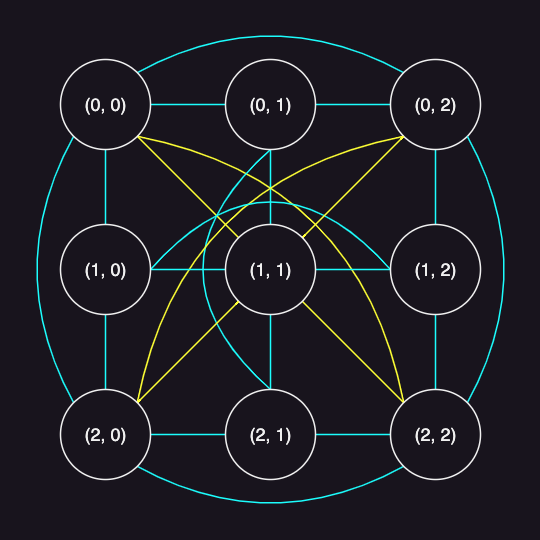
In the context of a 3x3 Latin square, there are arcs between any two variables that are constrained by being in the same row or column. These arcs can be represented as follows:
- Same row: ((0, 0) -> (0, 1)), ((0, 0) -> (0, 2)), …
- Same column: ((0, 0) -> (1, 0)), ((0, 0) -> (2, 0)), …
The following figure is a node graph of a 3x3 Latin square. Each node represents a variable, and each line represents a binary constraint (an arc).

Arc consistency is a property of binary constraints between two variables in a CSP.
In technical terms:
An arc
(X -> Y)is consistent if for every value in the domain ofX, there is at least one compatible value in the domain ofYthat satisfies the constraint betweenXandY.
Arc consistency is an important concept because it helps prune the search space by eliminating values from the variable domains that can’t possibly lead to a solution. This significantly speeds up the solving process. The most common algorithm used to enforce arc consistency is AC-3, which we’ll discuss later.
Backtracking
The idea of backtracking is to build a solution incrementally, abandoning a path as soon as it becomes clear that there is no solution found. It’s not just used in constraint satisfaction problems. You’ll also see it in problems like puzzles and combinatorial search, where efficiently exploring all possible options really matters.
Here’s how it works, step by step:
- Start from an empty or initial state.
- Make a choice to move forward (pick a possible next step).
- If the current path is valid, continue exploring deeper.
- If you hit a dead-end (no valid moves or constraints are violated), undo the last choice (backtrack) and try another option.
- Repeat this process until you find a complete solution or exhaust all possibilities.
Basically, it’s a recursive algorithm.
Let’s encode this idea in Python.
Here’s a naive implementaion to solve a 5x5 Latin square:
# backtrack.py
"""
Naive backtracking search for Latin square CSP.
"""

from csp import CSP
from latin_square import create_latin_square, print_latin_square


def backtrack(assignment: dict, csp: CSP) -> dict | None:
    if len(assignment) == len(csp.variables):  # Return assignment if complete
        return assignment

    variable = select_unassigned_variable(assignment, csp)
    for value in get_domain_values(variable, assignment, csp):
        new_assignment = assignment.copy()
        new_assignment[variable] = value
        if is_consistent(new_assignment, csp.constraints):
            result = backtrack(new_assignment, csp)  # Recur with the new assignment
            if result:
                return result  # Solution found
    return None  # No solution found


def select_unassigned_variable(assignment: dict, csp: CSP):
    for variable in csp.variables:
        if variable not in assignment:
            return variable
    return None


def get_domain_values(variable, assignment: dict, csp: CSP) -> list:
    """
    Get the domain values for a variable without specific ordering.
    """
    return csp.domains[variable]


def is_consistent(assignment: dict, constraints: list) -> bool:
    """
    Check if the assignment is consistent with the constraints for Latin square.
    """
    # Check if any constraints are violated
    for var1, var2 in constraints:
        if var1 in assignment and var2 in assignment:
            if assignment[var1] == assignment[var2]:
                return False  # assignment is not consistent
    return True  # assignment is consistent


if __name__ == "__main__":
    SIZE = 5
    latin_square_csp = create_latin_square(size=SIZE)

    # assignment is a dictionary that maps variable to value
    assignment = backtrack({}, latin_square_csp)
    if assignment:
        print_latin_square(assignment)
    else:
        print("No solution found.")
Here’s how it flows.
The backtrack function tries to assign values to variables one by one:
- Base case: If every variable has a value (assignment complete), return the solution.
select_unassigned_variable: Pick the next unassigned variable.get_domain_values: Try every possible value from the variable’s domain.is_consistent: After each assignment, check if constraints (no conflicts) are satisfied.- Recursion: Continue with this new assignment; if it leads to a dead end, backtrack.
Running this code will output:
Latin square Solution for 5x5:
1 2 3 4 5
2 1 4 5 3
3 4 5 1 2
4 5 2 3 1
5 3 1 2 4
Below is a visual breakdown of the step-by-step process for solving a 5x5 Latin square:

Testing
To verify the solution:
# test_latin_square.py
from backtrack import backtrack
from latin_square import create_latin_square


def check_rows(solution: dict[tuple[int, int], int], size: int) -> bool:
    """Check if each row contains unique numbers from 1 to size."""
    for r in range(size):
        row_values = {solution[(r, c)] for c in range(size)}
        if row_values != set(range(1, size + 1)):
            return False
    return True


def check_cols(solution: dict[tuple[int, int], int], size: int) -> bool:
    """Check if each column contains unique numbers from 1 to size."""
    for c in range(size):
        col_values = {solution[(r, c)] for r in range(size)}
        if col_values != set(range(1, size + 1)):
            return False
    return True


def test_latin_square():
    """Test the Latin square CSP with different sizes."""
    for size in range(5, 10):
        latin_square = create_latin_square(size)
        solution = backtrack({}, latin_square)

        assert solution is not None, "Backtrack function should find a solution"
        assert len(solution) == size * size, "Solution should have size * size assignments"

        # Verify constraints
        assert check_rows(solution, size), "Row constraint violated"
        assert check_cols(solution, size), "Column constraint violated"
You can run it using pytest:
pytest test_latin_square.py
Limitation
The problem with this naive implementation is that as the size of the square increases, the number of backtrack calls grows dramatically, leading to a huge increase in computation.
To illustrate this, we can get a sense of the computational effort by counting how many times backtrack is called.
Here’s the result for Latin squares ranging from size 1 to 10:
| Size | Backtrack Calls |
|---|---|
| 1 | 2 |
| 2 | 5 |
| 3 | 11 |
| 4 | 17 |
| 5 | 38 |
| 6 | 63 |
| 7 | 132 |
| 8 | 65 |
| 9 | 303 |
| 10 | 1465 |
Line graph:

Meanwhile, one interesting observation is that a larger problem doesn’t always mean more backtracking. For example, solving the 8x8 grid actually required fewer backtrack calls than the 7x7. This suggests that problem difficulty isn’t just about size. Some instances are just naturally friendlier to the search process.
Back to the main point, as you can see, the computational cost increases rapidly, even for moderately larger squares.
Moreover, the problem becomes even harder when additional constraints are added. For example, consider a Diagonal Latin square, where elements along both the main diagonal and the anti-diagonal must also be unique.
We can model this diagonal Latin square by adding more constraints as follows:
# latin_square.py
...


def create_diagonal_latin_square(size: int) -> CSP:
    """
    Create a CSP for diagonal Latin square (DLS) of given size.
    """
    csp = create_latin_square(size)

    # Add constraints for diagonal elements
    for i in range(size):
        for k in range(i + 1, size):
            # Main diagonal constraints
            csp.constraints.append(((i, i), (k, k)))
            # Anti-diagonal constraints
            csp.constraints.append(((i, size - 1 - i), (k, size - 1 - k)))
    return csp
The following figure is a node graph of a 3x3 diagonal Latin square.
In fact, diagonal Latin squares are impossible for certain sizes, such as 2 and 3.
As as result, adding these diagonal constraints causes the number of backtracking calls to skyrocket:
| Size | Backtrack Calls | Solution Found |
|---|---|---|
| 1 | 2 | Yes |
| 2 | 5 | No |
| 3 | 28 | No |
| 4 | 30 | Yes |
| 5 | 191 | Yes |
| 6 | 1658 | Yes |
| 7 | 87944 | Yes |
Below is a visual explanation of how many steps are added to solve a 5x5 Latin square compared to the previous example:

This happens because the search space becomes much more restricted, making it harder for the algorithm to find valid placements without conflict. With more constraints, the algorithm has to backtrack more frequently.
Adding unary constraints can also make the problem significantly harder as well.
For instance, let’s force the main diagonal elements to follow a specific sequence:
# latin_square.py
...


def create_diagonal_latin_square_with_unary_constraints(size: int) -> CSP:
    """
    Create a CSP for diagonal Latin square (DLS) of given size with additional unary constraints.
    """
    csp = create_diagonal_latin_square(size)
    # Add unary constraints to make problem harder
    for i in range(size):
        csp.domains[(i, i)] = {i + 1}
    return csp
These unary constraints further reduce the available choices for key variables right from the beginning, which leads to more failures during search and thus more backtracking.
| Size | Backtrack Calls | Solution Found |
|---|---|---|
| 1 | 2 | Yes |
| 2 | 3 | No |
| 3 | 10 | No |
| 4 | 56 | Yes |
| 5 | 400 | Yes |
| 6 | 44534 | Yes |
Once you throw in those diagonal and unary constraints, even a 7x7 Latin square becomes brutally slow for naive backtracking. On most modern PCs, you’ll be stuck waiting who-knows-how-long for a solution.
To address these challenges and improve efficiency, we will enforce arc consistency by using AC-3 algorithm.
Update the test to verify the diagonal Latin square with unary constraints:
# test_latin_square.py
...


def check_main_diagonal(solution: dict[tuple[int, int], int], size: int) -> bool:
    """Check if the main diagonal contains unique numbers from 1 to size."""
    diag_values = {solution[(i, i)] for i in range(size)}
    # For the specific DLS generated by create_dls, the diagonal is fixed
    expected_diag_values = {i + 1 for i in range(size)}
    return diag_values == expected_diag_values


def check_anti_diagonal(solution: dict[tuple[int, int], int], size: int) -> bool:
    """Check if the anti-diagonal contains unique numbers from 1 to size."""
    anti_diag_values = {solution[(i, size - 1 - i)] for i in range(size)}
    return len(anti_diag_values) == size and all(1 <= v <= size for v in anti_diag_values)


def check_unary_constraints(solution: dict[tuple[int, int], int], size: int) -> bool:
    """Check if the unary constraints are satisfied."""
    for i in range(size):
        if (i, i) in solution:
            if solution[(i, i)] != i + 1:
                return False
    return True


def test_latin_square_diagonal_with_unary_constraints():
    """Test the Latin square CSP with diagonal constraints and unary constraints."""
    for size in range(4, 7):
        latin_square = create_diagonal_latin_square_with_unary_constraints(size)
        solution = backtrack({}, latin_square)

        assert solution is not None, "Backtrack function should find a solution"
        assert len(solution) == size * size, "Solution should have size * size assignments"

        # Verify constraints
        assert check_rows(solution, size), "Row constraint violated"
        assert check_cols(solution, size), "Column constraint violated"
        assert check_main_diagonal(solution, size), "Main diagonal constraint violated"
        assert check_anti_diagonal(solution, size), "Anti-diagonal constraint violated"
        assert check_unary_constraints(solution, size), "Unary constraint violated"
AC-3 Algorithm
The AC-3 is an algorithm used in constraint satisfaction problems to enforce arc consistency. It processes all arcs in the problem, removing inconsistent values from variable domains until all arcs are consistent — or until it detects that no solution is possible. By reducing the domains early, AC-3 helps prune the search space, leading to fewer backtracks and faster solutions during search.
In Python, it can be implemented as follows:
# ac3.py
from csp import CSP


def ac3(csp: CSP) -> bool:
    """
    Enforce arc consistency using AC-3 algorithm.
    """
    queue = csp.constraints.copy()  # Initialize the queue with all constraints
    while queue:
        (x, y) = queue.pop(0)
        if arc_reduce(x, y, csp):
            if not csp.domains[x]:
                return False  # No solution found
            for z in get_neighbors(x, csp.constraints):
                if z != y:
                    queue.append((z, x))
    return True


def arc_reduce(x, y, csp: CSP) -> bool:
    """
    Make variable x arc-consistent with variable y.
    Return True if domain of x is reduced, False otherwise.
    """
    changed = False
    for vx in csp.domains[x].copy():
        satisfied = False
        # Find a value in the domain of y that satisfies the constraint
        for vy in csp.domains[y]:
            if vx != vy:
                satisfied = True
                break
        if not satisfied:
            csp.domains[x].remove(vx)
            changed = True
    return changed


def get_neighbors(variable, constraints: list) -> list:
    """
    Get all neighbors of a variable based on the constraints.
    """
    neighbors = []
    for var1, var2 in constraints:
        if var1 == variable:
            neighbors.append(var2)
        elif var2 == variable:
            neighbors.append(var1)
    return neighbors
In the code above:
ac3(csp)initializes a queue with all binary constraints and processes them one by one. For each arc(X -> Y), it checks whether the domain ofXcan be reduced based onYusingarc_reduce(x, y, csp).arc_reduce(x, y, csp)attempts to prune inconsistent values fromX’s domain. If a value ofXcannot be matched with any value ofY, that value is removed.get_neighbors(variable, constraints)returns all variables that share a constraint with the given variable, ensuring that after reducingX’s domain, related arcs are re-added to the queue for rechecking.
If any domain becomes empty during this process, the algorithm returns False, indicating that no solution is possible under the current assignments.
Otherwise, it returns True once all arcs are consistent.
Here are two main ways to apply the AC-3 algorithm:
- Initial pruning: at the start of the problem before starting the search.
- Maintaining Arc Consistency (MAC): during the search itself.
Initial Pruning
We can apply AC-3 to the CSP to prune the search space before staring the search. This preprocessing step can help reduce the number of backtracks needed during the actual search in advance:
latin_square_csp = create_diagonal_latin_square_with_unary_constraints(size=5)

# assignment is a dictionary that maps variable to value
ac3(latin_square_csp)  # Enforce arc consistency before backtracking (initial pruning)
assignment = backtrack({}, latin_square_csp)
if assignment:
    print_latin_square(assignment)
else:
    print("No solution found.")
Pros:
- Easy to implement.
- Can eliminate many early inconsistencies.
- Reduces search space before starting.
Cons:
- Only detects inconsistencies before search.
- Cannot prevent failures that arise during search.
As an example, the table below shows how the domains of each variable in a 3×3 Latin square are refined before and after applying the AC-3 algorithm at the beginning.
| Variable | Before AC-3 | After AC-3 |
|---|---|---|
| (0, 0) | {1} | ∅ |
| (0, 1) | {1, 2, 3} | {1, 3} |
| (0, 2) | {1, 2, 3} | {1} |
| (1, 0) | {1, 2, 3} | {1, 3} |
| (1, 1) | {2} | {2} |
| (1, 2) | {1, 2, 3} | {1, 2} |
| (2, 0) | {1, 2, 3} | {1, 2} |
| (2, 1) | {1, 2, 3} | {1, 2} |
| (2, 2) | {3} | {3} |
As a result, we can immediately detect that the problem has no solution because one of the variables (0, 0) has an empty domain after constraint propagation, meaning no valid value can be assigned without violating the Latin square constraints.
The number of backtracking calls when solving a diagonal Latin square with unary constraints, with AC-3 applied before backtracking:
| Size | Backtrack Calls | Solution Found |
|---|---|---|
| 1 | 2 | Yes |
| 2 | 2 | No |
| 3 | 1 | No |
| 4 | 21 | Yes |
| 5 | 48 | Yes |
| 6 | 864 | Yes |
| 7 | 155466 | Yes |
| 8 | 111898 | Yes |
When compared to the result without AC-3, the difference in backtracking calls becomes increasingly noticeable as the grid size grows.
Maintaining Arc Consistency (MAC)
We can also maintain arc consistency dynamically during the backtracking process. After each variable assignment, we enforce arc consistency again, ensuring that every partial assignment remains as consistent as possible before proceeding further. This approach can help reduce the need for deep backtracking by detecting dead-ends earlier:
def backtrack(assignment: dict, csp: CSP) -> dict | None:
    if len(assignment) == len(csp.variables):  # Return assignment if complete
        return assignment

    variable = select_unassigned_variable(assignment, csp)
    for value in list(get_domain_values(variable, assignment, csp)):
        new_assignment = assignment.copy()
        new_assignment[variable] = value
        if is_consistent(new_assignment, csp.constraints):
            domains = csp.domains.copy()  # Save the original domains
            if ac3(csp):  # Enforce arc consistency
                result = backtrack(new_assignment, csp)  # Recur with the new assignment
                if result:
                    return result  # Solution found
            csp.domains = domains  # Restore the original domains
    return None  # No solution found
Pros:
- Continuously prunes domains after each assignment.
- Detects dead-ends early.
- Leads to fewer backtracks and deeper pruning.
Cons:
- More computational overhead at each step.
- Slightly more complex to implement and manage.
The number of backtrack calls when using MAC isn’t much different from that of initial pruning. In fact, using MAC can actually be slower than simply doing that initial pruning. You can see this for yourself by comparing the processing time of both versions of the code. So, running AC-3 just once at the start is more than enough to significantly improve performance for our Latin square example.
The takeaway here is that while it’s possible to apply AC-3 at the beginning and also during the backtracking process, it’s not free. It comes with a computational cost. And sometimes, that extra overhead outweighs any benefit it might bring.
We will use initial pruning for the rest of the examples.
To further improve search efficiency, we can use heuristics.
Heuristics
Heuristics are strategies used to make better decisions during search — like which variable to pick next or which value to try first. Instead of going through every possibility blindly, heuristics aim to cut down the search space and avoid dead ends early.
Three heuristics we’ll look at:
- Least Constraining Values (LCV)
- Minimum Remaining Values (MRV)
- Degree
Least Constraining Values (LCV)
The least constraining value (LCV) heuristic suggests trying the value that rules out the fewest choices for the neighboring (constrained) unassigned variables. The goal is to keep options open for future assignments, increasing the chance of finding a solution without backtracking.
This requires calculating, for each potential value of the current variable, how many choices would be eliminated for its unassigned neighbors.
(Previosuly, the get_domain_values just returns all domain values for a variable.)
For this, we will update the get_domain_values function:
...

def get_domain_values(variable, assignment: dict, csp: CSP) -> list:
    """
    Order domain values using the Least Constraining Values (LCV) heuristic.
    Returns values sorted by the number of choices they rule out for neighboring variables.
    """
    neighbors = get_neighbors(variable, csp.constraints)
    unassigned_neighbors = [n for n in neighbors if n not in assignment]

    value_counts = []
    for value in csp.domains[variable]:
        constraint_count = 0
        for unassigned_neighbor in unassigned_neighbors:
            if value in csp.domains[unassigned_neighbor]:
                constraint_count += 1
        value_counts.append((value, constraint_count))

    # Sort values by their constraint count (ascending)
    value_counts.sort(key=lambda x: x[1])

    # NOTE The first item is the least constraining value (that rules out the least number of choices for neighboring variables)
    return [value for value, _ in value_counts]

def get_neighbors(variable, constraints: list) -> list:
    """
    Get all neighbors of a variable based on the constraints.
    """
    neighbors = []
    for var1, var2 in constraints:
        if var1 == variable:
            neighbors.append(var2)
        elif var2 == variable:
            neighbors.append(var1)
    return neighbors
With LCV heuristic used (alongside AC-3), the number of backtrack calls significantly improves:
| Size | Backtrack Calls | Solution Found |
|---|---|---|
| 1 | 2 | Yes |
| 2 | 2 | No |
| 3 | 1 | No |
| 4 | 20 | Yes |
| 5 | 36 | Yes |
| 6 | 905 | Yes |
| 7 | 854 | Yes |
| 8 | 5588 | Yes |
Note the drastic drop in backtrack calls for size 7 compared to the previous 155466 without LCV. This demonstrates how combining constraint propagation and value ordering (like LCV) can make a huge difference in search efficiency.
Minimum Remaining Values (MRV)
The minimum remaining values (MRV) heuristic (a.k.a. “most constrained variable” heuristic) suggests selecting the variable with the fewest legal values remaining in its domain. The intuition is that if a variable has only one or very few valid choices left, it’s better off to assign it now. This might lead to an immediate failure if no values are legal, allowing for quick backtracking.
For this, we will update the select_unassigned_variable function:
...

def select_unassigned_variable(assignment: dict, csp: CSP) -> tuple | None:
    """Select the unassigned variable with the fewest remaining legal values (MRV)."""
    variable = None
    minimum_remaining_values = float("inf")
    for candidate_variable in csp.variables:
        if candidate_variable not in assignment:
            num_remaining_values = len(csp.domains[candidate_variable])
            if num_remaining_values < minimum_remaining_values:
                minimum_remaining_values = num_remaining_values
                variable = candidate_variable  # Update the best variable found so far
    return variable
With MRV heuristic used (alongside AC-3):
| Size | Backtrack Calls | Solution Found |
|---|---|---|
| 1 | 2 | Yes |
| 2 | 1 | No |
| 3 | 1 | No |
| 4 | 20 | Yes |
| 5 | 40 | Yes |
| 6 | 711 | Yes |
| 7 | 22164 | Yes |
| 8 | 91113 | Yes |
While MRV consistently improves performance, it results in more backtracking calls than LCV when solving larger Latin squares.
Degree
The degree heuristic suggests selecting the variable involved in the largest number of constraints with other unassigned variables.
In a Latin square, each cell (r, c) is constrained by the other N-1 cells in its row and the other N-1 cells in its column. The degree heuristic tries to pick the variable that constrains the most remaining choices.
Here’s the degree heuristic implemented version:
...

def select_unassigned_variable(assignment: dict, csp: CSP) -> tuple | None:
    """
    Select the unassigned variable using degree heuristic.
    This heuristic selects the variable that is involved in the largest number of constraints.
    """
    max_degree: int = -1
    selected_variable = None
    for var in csp.variables:
        if var not in assignment:
            num_neighbors = len(get_neighbors(var, csp.constraints))
            if num_neighbors > max_degree:
                max_degree = num_neighbors
                selected_variable = var  # Update the selected variable
    return selected_variable

def get_neighbors(variable, constraints: list) -> list:
    """
    Get all neighbors of a variable based on the constraints.
    """
    neighbors = []
    for var1, var2 in constraints:
        if var1 == variable:
            neighbors.append(var2)
        elif var2 == variable:
            neighbors.append(var1)
    return neighbors
With degree heuristic used (alongside AC-3):
| Size | Backtrack Calls | Solution Found |
|---|---|---|
| 1 | 2 | Yes |
| 2 | 2 | No |
| 3 | 2 | No |
| 4 | 17 | Yes |
| 5 | 31 | Yes |
| 6 | 39 | Yes |
| 7 | 651 | Yes |
| 8 | 568577 | Yes |
The degree heuristic performs really well for Latin squares up to size 7, but after that, the computation cost shoots up significantly.
The key insight here is that there’s no one-size-fits-all solution—even for a single problem type like Latin squares. Different heuristics behave differently depending on the size and complexity of the instance. That’s why it’s important to experiment with various strategies rather than sticking to just one. What works well for a 7x7 grid might fall apart on an 8x8.
LCV + MRV + Degree
Finally, let’s put all the heuristics together—LCV, MRV, and the Degree heuristic to see how well they perform when combined in a backtracking search.
Here’s the code that integrates all three:
from ac3 import ac3
from csp import CSP
from latin_square import create_diagonal_latin_square_with_unary_constraints, print_latin_square


def backtrack(assignment: dict, csp: CSP) -> dict | None:
    if len(assignment) == len(csp.variables):  # Return assignment if complete
        return assignment

    variable = select_unassigned_variable(assignment, csp)
    for value in get_domain_values(variable, assignment, csp):
        new_assignment = assignment.copy()
        new_assignment[variable] = value
        if is_consistent(new_assignment, csp.constraints):
            result = backtrack(new_assignment, csp)  # Recur with the new assignment
            if result:
                return result  # Solution found
    return None  # No solution found


def select_unassigned_variable(assignment: dict, csp: CSP) -> tuple | None:
    """
    Select unassigned variable using MRV (Minimum Remaining Values) heuristic
    with Degree heuristic as a tie-breaker.
    """
    unassigned_vars = []
    minimum_remaining_values: float = float("inf")

    # First pass: find all variables with minimum remaining values
    for var in csp.variables:
        if var not in assignment:
            num_remaining_values = len(csp.domains[var])
            if num_remaining_values < minimum_remaining_values:
                minimum_remaining_values = num_remaining_values
                unassigned_vars = [var]
            elif num_remaining_values == minimum_remaining_values:
                unassigned_vars.append(var)

    # If only one variable with minimum remaining values, return it
    if len(unassigned_vars) == 1:
        return unassigned_vars[0]

    # Use degree heuristic as tie-breaker
    max_degree: int = -1
    selected_variable = None
    for var in unassigned_vars:
        num_neighbors = len(get_neighbors(var, csp.constraints))
        if num_neighbors > max_degree:
            max_degree = num_neighbors
            selected_variable = var

    return selected_variable


def get_domain_values(variable, assignment: dict, csp: CSP) -> list:
    """
    Order domain values using the Least Constraining Values (LCV) heuristic.
    Returns values sorted by the number of choices they rule out for neighboring variables.
    """
    neighbors = get_neighbors(variable, csp.constraints)
    unassigned_neighbors = [n for n in neighbors if n not in assignment]

    value_counts = []
    for value in csp.domains[variable]:
        constraint_count = 0
        for unassigned_neighbor in unassigned_neighbors:
            if value in csp.domains[unassigned_neighbor]:
                constraint_count += 1
        value_counts.append((value, constraint_count))

    # Sort values by their constraint count (ascending)
    value_counts.sort(key=lambda x: x[1])

    # Return values ordered from least constraining to most constraining
    return [value for value, _ in value_counts]


def is_consistent(assignment: dict, constraints: list) -> bool:
    """
    Check if the assignment is consistent with the constraints for Latin square.
    """
    # Check if any constraints are violated
    for var1, var2 in constraints:
        if var1 in assignment and var2 in assignment:
            if assignment[var1] == assignment[var2]:
                return False  # assignment is not consistent
    return True  # assignment is consistent


def get_neighbors(variable, constraints: list) -> list:
    """
    Get all neighbors of a variable based on the constraints.
    """
    neighbors = []
    for var1, var2 in constraints:
        if var1 == variable:
            neighbors.append(var2)
        elif var2 == variable:
            neighbors.append(var1)
    return neighbors

if __name__ == "__main__":
    latin_square_csp = create_diagonal_latin_square_with_unary_constraints(size=5)
    ac3(latin_square_csp)
    assignment = backtrack({}, latin_square_csp)
    if assignment:
        print_latin_square(assignment)
    else:
        print("No solution found.")
The number of backtrack calls of all heuristics combined:
| size | Backtrack Calls | Solution Found |
|---|---|---|
| 1 | 2 | Yes |
| 2 | 1 | No |
| 3 | 1 | No |
| 4 | 17 | Yes |
| 5 | 26 | Yes |
| 6 | 49 | Yes |
| 7 | 91 | Yes |
| 8 | 475 | Yes |
You’ll notice a big drop in the number of backtrack calls and not just that, it also cuts down the actual processing time if you run the code.
Comparisons
The graph below compares six different approaches to solve diagonal Latin square with unary constraints.
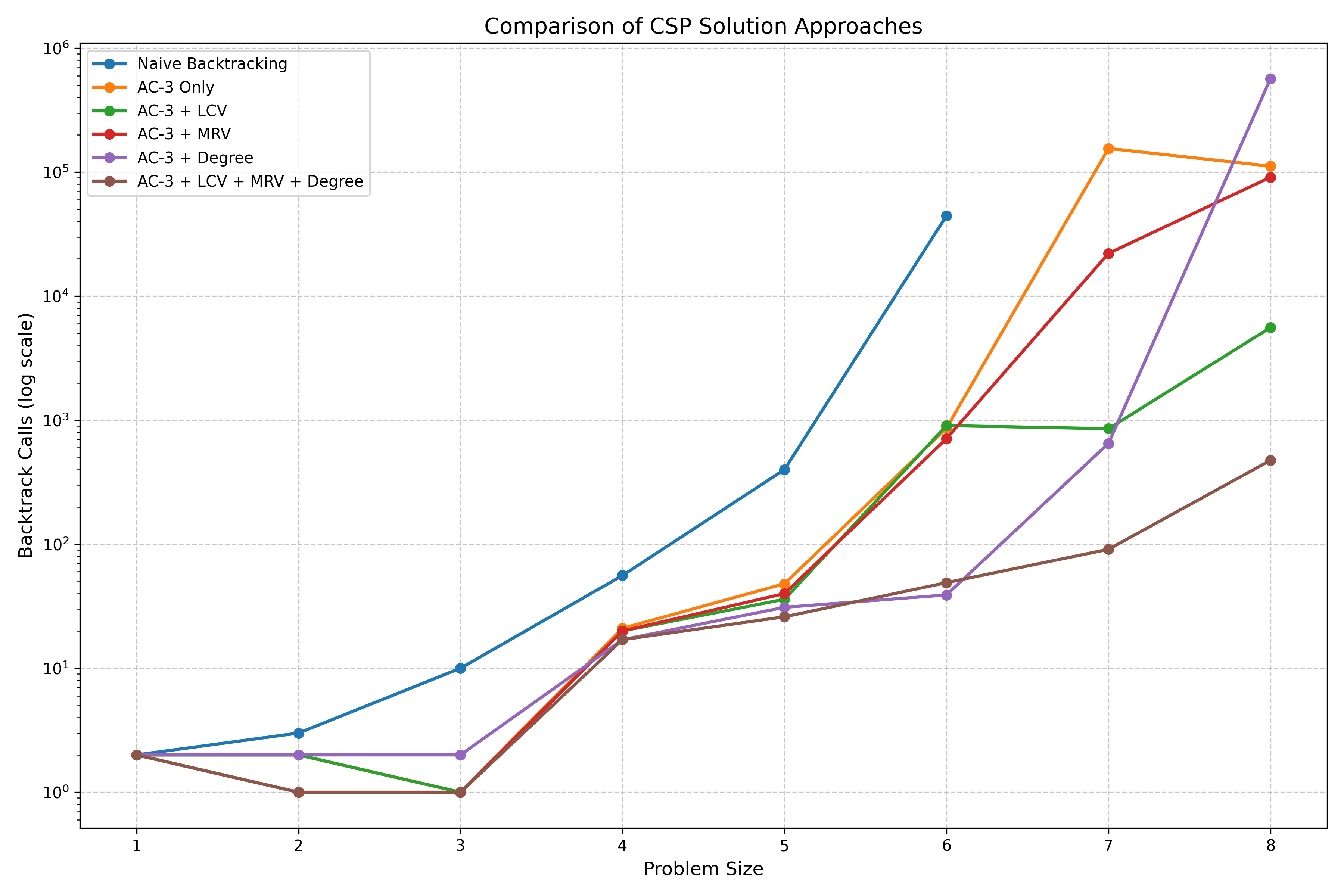
The key insight is that the logarithmic scale really highlights the performance differences. It shows that by combining advanced heuristics, you can solve larger Latin squares with a huge drop in computational effort.
Conclusion
Keep in mind that the number of backtrack calls is just one way to measure how efficient the search is. Heuristics can definitely help guide the search more intelligently, but figuring out the best move at every step can take extra computational overhead. So even if your heuristic seems to be reducing backtracking, if it’s working too hard behind the scenes, it might actually be slowing things down overall.