Systematic Evaluation for Information Retrieval: MAP and nDCG

The effectiveness (or accuracy) of an information retrieval system refers to how well it ranks relevant documents higher than non-relevant ones. Evaluating this effectiveness is important because it allows us to compare different algorithms, helping researchers and developers figure out which ideas and methods actually work better.

So, how do we measure it? Since information retrieval is fundamentally an empirical problem, its effectiveness has to be judged by users in some way. One obvious way is to look at what real users do. Metrics like click-through rate (CTR) and conversion rate fall into this category. These are often called online metrics. A/B testing is a popular way to compare different systems using this kind of data.

However, online experiments require deploying systems to actual users, which isn’t always practical or even possible in research settings. This is where systematic approaches based on offline metrics come in.

Cranfield Evaluation Methodology

Cranfield evaluation methodology is a framework for systematically evaluating the effectiveness of information retrieval systems, developed in the 1960s by Cyril Cleverdon at Cranfield University.

This methodology is built upon three key components:

• A collection of documents: a standardized set of documents to search against.
• A set of sample queries: representative queries that simulate user needs.
• Human-judged relevance judgments: a definitive list of which documents are considered relevant for each query.

Note that relevance judgments is by far the most important and the most labor-intensive part of the evaluation since they rely on human assessors. A common strategy to manage this is pooling, where assessors only judge a subset of results pulled together from several existing systems. However, this approach can introduce selection bias. If a new system retrieves relevant documents that never made it into the pool, those documents remain unjudged, and the system ends up being unfairly penalized.

Once we have all three components, the question becomes: how do we quantify the effectiveness?

Precision and Recall

Precision and recall are core metrics to quantify the effectiveness:

• Precision: Of all the documents the system retrieved, how many were actually relevant?
• Recall: Of all the relevant documents, how many did the system retrieve?

These concepts can be illustrated using a confusion matrix:

	Retrieved	Not Retrieved
Relevant	True Positive	False Negative
Not Relevant	False Positive	True Negative

From this matrix, precision and recall are defined as follows:

• Precision = $\frac{\text{Number of relevant documents retrieved}}{\text{Total number of documents retrieved}}$ = $\frac{TP}{TP + FP}$
• Recall = $\frac{\text{Number of relevant documents retrieved}}{\text{Total number of relevant documents in the collection}}$ = $\frac{TP}{TP + FN}$

Here’s an example.

Suppose we have a small test collection of 10 documents about software:

Document ID	Title
d1	Mastering Design Patterns in Python
d2	Writing Unit Tests with pytest
d3	Introduction to TypeScript
d4	Refactoring Legacy Codebases
d5	The Practical Test Pyramid
d6	Code Review Best Practices
d7	SQL Optimization Techniques
d8	Static Analysis with ruff
d9	Principles of Agile Development
d10	Test-Driven Development Explained

Our query is “software testing practices”

A human evaluator goes through the entire collection and determines which documents are relevant to the query:

Document ID	Title	Relevant
d1	Mastering Design Patterns in Python	0
d2	Writing Unit Tests with pytest	1
d3	Introduction to TypeScript	0
d4	Refactoring Legacy Codebases	0
d5	The Practical Test Pyramid	1
d6	Code Review Best Practices	1
d7	SQL Optimization Techniques	0
d8	Static Analysis with ruff	1
d9	Principles of Agile Development	0
d10	Test-Driven Development Explained	1

So, there are a total of 5 relevant documents in the collection.

Now, let’s say our retrieval system returns these 4 documents for the query:

• d2: Writing Unit Tests with pytest
• d5: The Practical Test Pyramid
• d9: Principles of Agile Development
• d10: Test-Driven Development Explained

Out of these 4, three are actually relevant (d2, d5, d10), while one (d9) is a false alarm. So:

• Precision = 3 / 4 = 0.75
• Recall = 3 / 5 = 0.6

In Python:

retrieved_docs = ["d2", "d5", "d9", "d10"]
relevant_docs = ["d2", "d5", "d6", "d8", "d10"]


def get_precision(retrieved: list[str], relevant: list[str]) -> float:
    true_positives = len(set(retrieved) & set(relevant))
    false_positives = len(set(retrieved) - set(relevant))
    if (true_positives + false_positives) > 0:
        return true_positives / (true_positives + false_positives)
    return 0


def get_recall(retrieved: list[str], relevant: list[str]) -> float:
    true_positives = len(set(retrieved) & set(relevant))
    false_negatives = len(set(relevant) - set(retrieved))
    if (true_positives + false_negatives) > 0:
        return true_positives / (true_positives + false_negatives)
    return 0

precision = get_precision(retrieved_docs, relevant_docs)
recall = get_recall(retrieved_docs, relevant_docs)

print(f"Precision: {precision:.2f}")
print(f"Recall: {recall:.2f}")

Output:

Precision: 0.75
Recall: 0.60

In practice, we often use a cutoff at a fixed number of top-ranked results. For example:

• Precision@5 (P@5): The precision when considering only the top 5 retrieved documents.
• Recall@10 (R@10): The recall when considering only the top 10 results.

The ideal system would achieve a precision and recall of 1, meaning it retrieved all relevant documents and no non-relevant ones. However, these two metrics has a classic trade-off: increasing recall by retrieving more documents often leads to a decrease in precision, and vice-versa. To balance the two, we use the F-measure.

F-Measure

F-measure (or F-score) is a way to combine precision and recall into a single score. Instead of just simply averaging them like (P+R)/2, it ensures that both precision and recall matter. The formula is:

\[F_{\beta} = \frac{(\beta^2 + 1) \times \text{P} \times \text{R}}{(\beta^2 \times \text{P}) + \text{R}}\]

Here, the parameter $\beta$ lets you put more weight on recall (if $\beta>1$) or on precision (if $\beta<1$).

The most common variant is the F1-measure, which calculates the harmonic mean of the two:

\[F_{1} = \frac{2 \times \text{P} \times \text{R}}{\text{P} + \text{R}}\]

In Python:

def get_f_score(precision: float, recall: float, beta: float = 1.0) -> float:
    if (precision + recall) > 0:
        return (beta**2 + 1) * precision * recall / (beta**2 * precision + recall)
    return 0

With F1-measure, a system cannot achieve a high F1-score without having both reasonably high precision and high recall. For example,

Precision	Recall	$F_{1}$-score
0.5	0.5	0.5
0.9	0.1	0.18

Notice how the last row shows the penalty in action: even though precision is high (0.9), the low recall (0.1) drags the F1-score way down.

Limitation

The main drawback of F-measure is that it’s set-based so it ignores the order of results. A system that ranks the most relevant document at the top gets the same score as one that hides it at the last, even though the user experience is completely different.

To evaluate a ranked list, we need to consider the order of the results.

Precision-Recall (PR) Curve

The Precision–Recall (PR) curve shows how well a retrieval system balances precision and recall as you move down a ranked list of results. In simple terms, it helps you see whether the relevant documents are concentrated near the top (good) or scattered deeper in the list (not good).

We create the curve by plotting precision against recall at every rank position $k$.

Let’s walk through an example.

Suppose there are 8 relevant documents in total for a query, and our system manages to retrieve 6 of them within the top 10 results ($k$ = 10):

	Relevant
d1	1
d2	1
d3	1
d4	0
d5	1
d6	1
d7	0
d8	1
d9	0
d10	0

Now, to build the PR curve, we calculate precision and recall at each step:

	Relevant	Cumulative Relevant	Precision	Recall
d1	1	1	1/1	1/8
d2	1	2	2/2	2/8
d3	1	3	3/3	3/8
d4	0	3	3/4	3/8
d5	1	4	4/5	4/8
d6	1	5	5/6	5/8
d7	0	5	5/7	5/8
d8	1	6	6/8	6/8
d9	0	6	6/9	6/8
d10	0	6	6/10	6/8

When plotting the curve, we usually only take the points where a new relevant document appears so that the curve look smoother. That gives us the following (recall on the x-axis, precision on the y-axis):

	Precision	Recall
d1	1/1	1/8
d2	2/2	2/8
d3	3/3	3/8
d5	4/5	4/8
d6	5/6	5/8
d8	6/8	6/8

And visually:

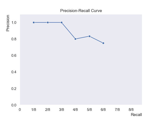
The curve makes it clear how front-loaded the relevant results are. If the curve stays high, the system surfaces relevant docs early. If it drops quickly, it means users would have to dig deeper before finding what they’re looking for.

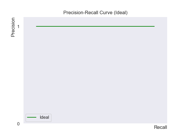
A system whose curve is higher and more to the right is better. Therefore, an ideal system would have a constant precision of 1.0 for all recall levels.

PR curves are especially useful when comparing multiple retrieval systems. Take the example below:

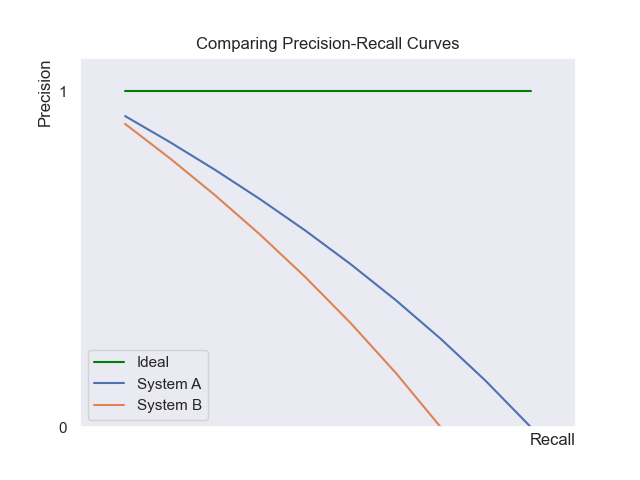
As System A’s curve is consistently above System B’s, A is clearly superior—it delivers better precision at every level of recall.

However, things get trickier when the curves cross. Take the example below:

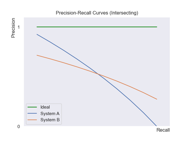
In this scenario, system A may have higher precision at low recall levels, while system B has higher precision at high recall levels. The better system depends on the user’s task. For example, a user doing a quick search might prefer System A’s high initial precision, whereas a researcher needing comprehensive results would prefer System B’s high recall.

Mean Average Precision (MAP)

Average Precision (AP)

When PR curves intersect, it’s useful to summarize performance with a single number. Average Precision (AP) does this by averaging the precision values at the ranks where relevant documents appear:

\[\text{AP}=\frac{1}{R}\sum_{k=i}^{N}P(k)Rel(k)\]

Where:

• $R$ is the total number of relevant documents for the query.
• $N$ is the total number of retrieved documents.
• $P(k)$ is the precision at the rank $k$.
• $Rel(k)$ is whether the document at rank $k$ is relevant (1) or not (0).

$R$ is NOT the number of retrieved relevant documents. If you were to divide by the number of retrieved relevant documents instead, you’d give an unfair advantage to a system that retrieves only a few documents. This would make the score look artificially high even if the system hardly retrieves anything useful.

AP is rank-sensitive: moving a relevant document higher in the list increases the score, while pushing it down lowers it. You can also think of it as a practical approximation of the area under the PR curve.

Let’s compute it for our example. We’ll take the precision at every rank where a relevant document shows up (d1, d2, d3, d5, d6, d8) and average them:

• Precision@d1 = 1/1
• Precision@d2 = 2/2
• Precision@d3 = 3/3
• Precision@d5 = 4/5
• Precision@d6 = 5/6
• Precision@d8 = 6/8

Now average these values:

\[AP = \frac{\frac{1}{1} + \frac{2}{2} + \frac{3}{3} + \frac{4}{5} + \frac{5}{6} + \frac{6}{8}}{8} \;\approx\; 0.67\]

In Python:

def get_average_precision(relevances: list[int], num_relevant: int) -> float:
    """
    Compute Average Precision (AP) for a single query.
    """
    if num_relevant == 0:
        return 0.0  # edge case: no relevant docs for this query

    precisions = []
    relevant_found = 0
    for k, rel in enumerate(relevances, start=1):  # rank positions start at 1
        if rel == 1:
            relevant_found += 1
            precision_at_k = relevant_found / k
            precisions.append(precision_at_k)

    return sum(precisions) / num_relevant


# Example usage
relevances = [1, 1, 1, 0, 1, 1, 0, 1, 0, 0]  # system output (10 results)
num_relevant = 8  # total relevant docs

AP = get_average_precision(docs, num_relevant)
print("Average Precision:", AP)

Average Precision is great for judging performance on a single query, but it only tells part of the story. To really understand how well a system works, we need to evaluate it across many queries and then aggregate the results. That way, the score reflects overall performance rather than just one example.

Mean Average Precision (MAP)

Mean Average Precision (MAP) is simply the mean of the Average Precision (AP) scores across all queries in the test set:

\[\text{MAP}=\frac{1}{Q}\sum_{q=1}^{Q}\text{AP}(q)\]

Where $Q$ is the total number of queries.

It provides a single, comprehensive number that summarizes the system’s ranking quality.

An alternative is the Geometric Mean Average Precision (gMAP), which uses a geometric mean instead of an arithmetic one. The choice between MAP and gMAP depends on the evaluation goal:

• MAP (Arithmetic Mean): The final score is more heavily influenced by high AP scores. This means MAP gives more weight to performance on “easy” queries where the system does well. It is useful if the goal is to measure overall performance, particularly on popular queries that are often easier.
• gMAP (Geometric Mean): This average is more sensitive to low AP scores. Therefore, gMAP emphasizes performance on “difficult” queries where the system struggles. It is useful if the goal is to improve the system’s performance on its weakest queries.

Here’s an example. Suppose we evaluate three queries and get the following AP scores:

• Query 1: 1.0
• Query 2: 0.5
• Query 3: 0.1

Then:

• MAP = $\frac{1.0 + 0.5 + 0.1}{3} \approx 0.53$
• gMAP = $(1.0 \times 0.5 \times 0.1)^{1/3} \approx 0.37$

Here, MAP emphasizes the strong performance on Query 1, while gMAP penalizes the weak score on Query 3 more heavily.

Mean Reciprocal Rank (MRR)

For certain search tasks, there is only one correct or relevant document. This occurs in “known-item searches,” where a user wants to find a single, specific page (e.g., the Youtube homepage), or in some question-answering tasks where there is only one right answer.

In this scenario, the Average Precision calculation simplifies to the Reciprocal Rank:

\[\text{Reciprocal Rank} = \frac{1}{r}\]

where $r$ is the rank position of the single relevant documen. For example, if the document is at rank 1, the score is 1. If it’s at rank 2, the score is 0.5, and so on.

The Mean Reciprocal Rank (MRR) is the average of these reciprocal ranks across all queries.

Here’s an example. Suppose we evaluate three queries and the relevant document appears at:

• Query 1: Rank 1 → Reciprocal Rank = 1/1
• Query 2: Rank 3 → Reciprocal Rank = 1/3
• Query 3: Rank 2 → Reciprocal Rank = 1/2

Then

• MRR = $\frac{1/1 + 1/3 + 1/2}{3} \approx 0.61$

Limitation

MAP and MRR are built on the assumption of binary relevance judgments, either a document is relevant (1) or not (0). But in reality, some documents are highly relevant, while others are only marginally relevant.

Let’s revisit our earlier example with the query “software testing practices”:

Document ID	Title	Relevant
d1	Mastering Design Patterns in Python	0
d2	Writing Unit Tests with pytest	1
d3	Introduction to TypeScript	0
d4	Refactoring Legacy Codebases	0
d5	The Practical Test Pyramid	1
d6	Code Review Best Practices	1
d7	SQL Optimization Techniques	0
d8	Static Analysis with ruff	1
d9	Principles of Agile Development	0
d10	Test-Driven Development Explained	1

Here, documents like d2, d5, and d10 are highly relevant — they directly address testing practices. On the other hand, d6 and d8 are only somewhat relevant - they touch on quality practices but don’t focus on testing itself.

To handle this, we need a measure that accounts for graded relevance.

Normalized Discounted Cumulative Gain (nDCG)

Normalized Discounted Cumulative Gain (nDCG) is a metric for evaluating retrieval systems when relevance judgments are multi-level. It measures how good a ranking is by considering both the relevance and position.

In nDCG, relevance is usually graded on a scale from 1 to $r$ (where $r$ > 2). For example, if $r$ = 3, you might define:

• 1 = not relevant
• 2 = somewhat relevant
• 3 = highly relevant

The formula is:

\[\text{nDCG@}k=\frac{\text{DCG@}k}{\text{IDCG@}k}\]

Let’s walk through an example to see how this works.

Gain

The first step is assigning a gain value to each document, which is simply its relevance score:

\[G_i=Rel_i\]

Where $G_i$ is the gain of the result at position $i$.

Let’s take a simple example using a 3-level relevance scale ($r$ = 3). Suppose our system returns 5 results for a query q1, ranked from to to bottom:

Rank	Document	Relevance	Gain
1	d1	3 (highly relevant)	3
2	d2	2 (somewhat relevant)	2
3	d3	1 (not relevant)	1
4	d4	2 (somewhat relevant)	2
5	d5	3 (highly relevant)	3

So far, gain is just the raw relevance score.

Cumulative Gain (CG)

Cumulative Gain (CG) is the sum of gains up to rank $k$:

\[\text{CG@k}=\sum_{i=1}^{k}{G_i}\]

For our example:

Document	Gain	Cumulative Gain
d1	3	3
d2	2	3 + 2
d3	1	3 + 2 + 1
d4	2	3 + 2 + 1 + 2
d5	3	3 + 2 + 1 + 2 + 3

So,

\[\text{CG@5}=3+2+1+2+3=11\]

The problem with CG is that it ignores the rank order. If you change the top and bottom documents, the CG@5 is still 11. Clearly, that doesn’t reflect user experience because users care much more about the top results.

Discounted Cumulative Gain (DCG)

To make the metric rank-sensitive, the gain at each position is discounted by a logarithmic reduction factor (discount factor). The formula is:

\[\text{DCG@k}=\sum_{i=1}^{k}\frac{G_i}{\log_2(i+1)}={G_1}+\sum_{i=2}^{k}\frac{G_i}{\log_2(i+1)}\]

Here, the denominator, $\log_2(i+1)$, reduces the contribution of documents as their rank gets lower. This means a highly relevant document contributes more to the score if it is ranked higher.

For our example:

Document	Gain	Discount Factor
d1	3	1
d2	2	log3
d3	1	log4
d4	2	log5
d5	3	log6

So:

\[\text{DCG@}5=3+\frac{2}{\log3}+\frac{1}{\log4}+\frac{2}{\log5}+\frac{3}{\log6} \approx 6.78\]

To compute this with Python, we first define two dictionaries:

qrels_dict = {"q1": {"d1": 3, "d2": 2, "d3": 1, "d4": 2, "d5": 3}}
run_dict = {"q1": {"d1": 0.9, "d2": 0.8, "d3": 0.7, "d4": 0.6, "d5": 0.5}}

• qrels_dict: the relevance judgments for each query and document.
• run_dict: the system’s predicted ranking scores. The exact values don’t matter for DCG as long as they preserve the order since what we ultimately care about is the ranking of documents.

A function to compute DCG:

import math


def get_dcg(qrels_dict: dict, run_dict: dict, k: int, query: str) -> float:
    """
    Compute DCG@k for a specific query.
    """
    # Extract documents for the specific query
    query_qrels = qrels_dict.get(query, {})
    query_run = run_dict.get(query, {})

    # Sort documents by their scores in run_dict (descending order)
    sorted_docs = sorted(query_run.items(), key=lambda x: x[1], reverse=True)

    dcg = 0.0
    for i in range(min(k, len(sorted_docs))):
        doc_id = sorted_docs[i][0]
        relevance = query_qrels.get(doc_id, 0)  # default to 0 if doc not in qrels
        rank = i + 1
        if rank == 1:
            dcg += relevance  # no log discount for rank 1
        else:
            dcg += relevance / (math.log2(rank + 1))  # log base 2
    return dcg


qrels_dict = {"q1": {"d1": 3, "d2": 2, "d3": 1, "d4": 2, "d5": 3}}
run_dict = {"q1": {"d1": 0.9, "d2": 0.8, "d3": 0.7, "d4": 0.6, "d5": 0.5}}

dcg = get_dcg(qrels_dict, run_dict, 5, "q1")
print(f"{dcg:.2f}")

Output:

6.78

Now the ranking matters, but there’s still an issue. DCG scores aren’t directly comparable across queries. Imagine one query has only one relevant document and another has five. Even if both systems ranked perfectly, the DCG for the “easy” query (with lots of relevant docs) will naturally be higher. Without normalization, comparing those scores is unfair.

Normalized Discounted Cumulative Gain (nDCG)

To solve this, we normalize DCG by dividing it by the ideal DCG (IDCG):

\[\text{nDCG@}k=\frac{\text{DCG@}k}{\text{IDCG@}k}\]

Where IDCG is the DCG of an ideal ranking where all the most relevant documents are at the top.

This scales the score between 0 and 1: A system with nDCG = 1 means it produced the ideal ranking. And values below 1 tell you how close (or far) the system is from that ideal.

Suppose the ideal ordering is: [3, 3, 2, 2, 1] for our example:

Rank (k)	Gain	Discount Factor
1	3	1
2	3	log3
3	2	log4
4	2	log5
5	1	log6

(Note that the ideal ordering could also be [3, 3, 3, 3, 2] or even [3, 3, 3, 3, 3], depending on how many highly relevant documents exist in the collection.)

So:

\[\text{IDCG@}5=3+\frac{3}{\log3}+\frac{2}{\log4}+\frac{2}{\log5}+\frac{1}{\log6} \approx 7.14\]

Finally:

\[\text{nDCG@}5=\frac{\text{DCG}@5}{\text{IDCG}@5}=\frac{6.78}{7.14} \approx 0.95\]

In Python:

import math


def get_dcg(qrels_dict: dict, run_dict: dict, k: int, query: str) -> float:
    """
    Compute DCG@k for a specific query.
    """
    # Extract documents for the specific query
    query_qrels = qrels_dict.get(query, {})
    query_run = run_dict.get(query, {})

    # Sort documents by their scores in run_dict (descending order)
    sorted_docs = sorted(query_run.items(), key=lambda x: x[1], reverse=True)

    dcg = 0.0
    for i in range(min(k, len(sorted_docs))):
        doc_id = sorted_docs[i][0]
        relevance = query_qrels.get(doc_id, 0)  # default to 0 if doc not in qrels
        rank = i + 1
        if rank == 1:
            dcg += relevance  # no log discount for rank 1
        else:
            dcg += relevance / (math.log2(rank + 1))  # log base 2

    return dcg


def get_ndcg(qrels_dict: dict, run_dict: dict, k: int, query: str) -> float:
    """
    Compute nDCG@k for a specific query.
    """
    dcg = get_dcg(qrels_dict, run_dict, k, query)

    # Compute ideal DCG (iDCG)
    query_qrels = qrels_dict.get(query, {})
    ideal_relevances = sorted(query_qrels.values(), reverse=True)

    idcg = 0.0
    for i in range(min(k, len(ideal_relevances))):
        relevance = ideal_relevances[i]
        rank = i + 1
        if rank == 1:
            idcg += relevance
        else:
            idcg += relevance / (math.log2(rank + 1))

    if idcg == 0:
        return 0.0  # Avoid division by zero; if no relevant documents, nDCG is defined as 0

    ndcg = dcg / idcg

    return ndcg


qrels_dict = {"q1": {"d1": 3, "d2": 2, "d3": 1, "d4": 2, "d5": 3}}
run_dict = {"q1": {"d1": 0.9, "d2": 0.8, "d3": 0.7, "d4": 0.6, "d5": 0.5}}

ndcg = get_ndcg(qrels_dict, run_dict, 5, "q1")
print(f"{ndcg:.2f}")

Output:

0.95

In fact, there’s a Python library ranx that handles evaluation metrics like nDCG out of the box.

Here’s how you can compute nDCG@5 using ranx in just a few lines:

from ranx import Qrels, Run, evaluate

qrels_dict = {"q1": {"d1": 3, "d2": 2, "d3": 1, "d4": 2, "d5": 3}}
run_dict = {"q1": {"d1": 0.9, "d2": 0.8, "d3": 0.7, "d4": 0.6, "d5": 0.5}}

qrels = Qrels(qrels_dict)
run = Run(run_dict)

ndcg = evaluate(qrels, run, metrics="ndcg@5")
print(f"{ndcg:.2f}")

Limitation

When comparing two systems, looking only at the average nDCG score (or any single metric) isn’t enough. The question is: “How confident are we that the observed difference isn’t just because of the particular queries we happened to test?”

Imagine two systems:

• System A has an average score of 0.20
• System B has an average score of 0.40

At first glance, System B looks twice as good. But let’s dig deeper:

• Experiment 1 (low variance): System B beats System A on every single query. Here, it’s safe to say B is better.
• Experiment 2 (high variance): Some queries favor A, others favor B, and results swing wildly. The conclusion is much shakier.

This is where statistical significance tests come in.

Statistical Significance Testing

Statistical significance testing answers the question: “Is the observed difference real, or could it have happened by chance?”

Sign Test

One of the simplest approaches is the sign test. Instead of looking at averages, it counts how many times each system wins across queries.

Here’s an example with five queries and scores for two IR systems:

Query	System A	System B	Winner
q1	0.28	0.35	B
q2	0.30	0.20	A
q3	0.38	0.40	B
q4	0.29	0.33	B
q5	0.23	0.24	B

• Wins for System A: 1
• Wins for System B: 4

Here, System B clearly dominates by beating System A in 4 out of 5 queries. That’s a strong sign that B is better than A, at least on this test set.

Limitation

But here’s where things get tricky. Let’s extend the test set with four more queries:

Query	System A	System B	Winner
q1	0.28	0.35	B
q2	0.30	0.20	A
q3	0.38	0.40	B
q4	0.29	0.33	B
q5	0.23	0.24	B
q6	0.30	0.18	A
q7	0.21	0.24	B
q8	0.30	0.18	A
q9	0.34	0.18	A

• Wins for System A: 4
• Wins for System B: 5

Now, things don’t look so clear anymore. Even though System B has more wins overall, the margin is just a single query. With such small differences, it’s hard to say whether B is truly the better system or if the result is just due to chance. The sign test doesn’t capture how big the improvements are, only who won more often. To deal with this limitation, researchers often use more advanced significance tests, like the Wilcoxon signed-rank test.

Conclusion

For comparing different IR systems, MAP and nDCG are useful tools. They capture both relevance and ranking quality in a way that’s more informative than simple set-based measures.

But again, information retrieval is fundamentally an empirical problem. What a human assessor marks as “relevant” might not line up with what real users actually care about in the real-world context of search.

The takeaway is that to make reliable decisions, we need to evaluate across many queries. That’s how we avoid shaky averages and get confidence that one system is truly better than another.

References

• Evaluation measures (information retrieval) - Wikipedia
• Discounted cumulative gain - Wikipedia
• Text Retrieval and Search Engines by University of Illinois Urbana-Champaign