
Understanding BM25 in Text Retrieval
When you type a query into a search engine, it finds documents that contain your keywords. The problem is: how do you order those documents from most to least relevant?
Search engines use a ranking function to score document relevance. We write it as $f(q,d)$, where $q$ is the query and $d$ is a document. The higher the $f(q,d)$, the higher the document appears in the search results.
Although various methods exist to estimate document relevance, BM25 (Best Matching 25) is widely regarded as the most practical and effective ranking function for this task. It’s been around since the 90s, and despite newer ranking models, BM25 is still a strong baseline and often tough to beat in real-world applications.
The BM25 formula looks like this:
\[f(q,d) = \sum_{i=1}^{n}\frac{c(t_i,d)(k+1)}{c(t_i,d)+k(1-b+b\frac{|d|}{avdl})}(\log\frac{N+1}{df(t)+1}+1)\]At its heart, BM25 is just combining three heuristics:
- Term Frequency (TF)
- Inverse Document Frequencey (IDF)
- Document Length Normalization
In this post, I will explain each heuristic and show how they come together to form the BM25 formula.
Term Frequency (TF)
The simplest idea: if a query term appears more often in a document, that document is probably more relevant.
A TF-only ranking function’s formula can be represented as this:
\[f(q,d) = \sum_{i=1}^{n}TF(t_i,d)\]Where:
- $f(q,d)$ is the relevance score of document $d$ for query $q$.
- $\sum_{i=1}^{n}$ is the summation over all terms ($t_1$, $t_2$, …, $t_n$) in the query $q$.
- $TF(t_i,d)$ is the frequency score of query term $t_i$ in $d$.
Then how do we define $TF()$?
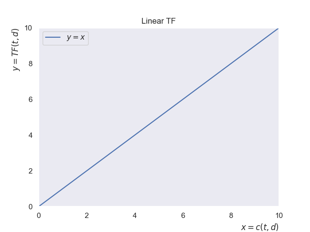
A naive TF is just to apply a linear count; $y=x$. Therefore:
\[TF(t,d) = c(t,d)\]Where $c(t,d)$ is the raw count of term t in document d.
Let’s see an example. Suppose we have two documents in our collection:
- d1: The Bank of Korea is expected to lower its benchmark interest rate next month.
- d2: A lower interest rate will be welcomed by indebted households.
Query: “korea interest rate”
Note that this query contains three terms: {$t_1$, $t_2$, $t_3$} = {“Korea”, “interest”, “rate”}
Under this linear application of the raw count, the scores are:
| documents | $f(q,d)$ |
|---|---|
| d1 | 3 |
| d2 | 2 |
Here, d2 contains two of the query terms—”interest” and “rate”—but misses “Korea”, and d1 matches all three.
This ordering makes intuitive sense: d1 fully matches the query, so it gets a higher score.
But there’s a problem: just repeating a term many times can inflate the score too much. This opens the door to what’s called term spamming. Term spamming is when a document unnaturally repeats certain keywords over and over to trick the ranking function into thinking it’s more relevant.
Suppose we add one more document to the collection:
- d3: The interest rate charged on loans is often higher than the interest rate paid on deposits.
With this new collection, the scores are:
| documents | $f(q,d)$ |
|---|---|
| d1 | 3 |
| d2 | 2 |
| d3 | 4 |
Obviously, this is not what we want. Instead, we’d prefer a system where repetition still helps, but each extra occurrence of the same word contributes less and less to the score. In other words, diminishing returns from repetition.
TF Transformation
One simple fix is to apply a sublinear transform like logarithmic transformation; $y=\log(x+1)$. Therefore:
\[TF(t,d) = \log(c(t,d)+1)\](1 is added to avoid $\log(0)$.)
This way, the impact of each extra occurrence shrinks.
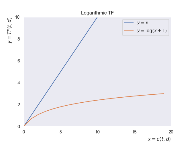
Still, it’s not perfect - TF is unbounded, meaning there’s no upper limit. A spammy document can still rack up arbitrarily high scores if it repeats a term enough times.
To improve it more, here comes a bounded transformation; $y=\frac{x(k+1)}{x+k}$. Therefore:
\[TF(t,d) = \frac{c(t,d)(k+1)}{c(t,d)+k}\]This function saturates at $(k+1)$, no matter how large $x$ gets. In other words, the function is upper-bounded by $k+1$.
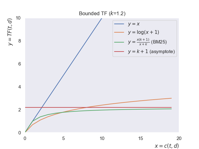
Not only is this transformation capped at $(k+1)$—which stops a single term’s frequency from completely dominating the score—it’s also flexible. The parameter $k$ controls how quickly the curve saturates:
- If $k=0$, it reduces to a simple binary scheme: any occurrence of the term contributes a score of 1, no matter how many times it appears.
- If $k$ is very large, the function behaves almost linearly, getting closer to the linear term frequency.
With this, our TF-based ranking function becomes:
\[f(q,d) = \sum_{i=1}^{n}\frac{c(t_i,d)(k+1)}{c(t_i,d)+k}\]This TF function can be implemented in Python like below:
def tf(term: str, document: str, k: float = 1.2) -> float:
    """
    Calculate TF score using bounded transformation.
    """
    # Apply some basic text normalization: 1. punctuation handling 2. lowercasing
    doc_terms = document.replace(".", " ").lower().split()
    term_count = doc_terms.count(term.lower())
    score = term_count * (k + 1) / (term_count + k)

    return score


def tf_ranking_function(query: str, document: str, k: float = 1.2) -> float:
    """
    Calculate TF score of a document with respect to a query.
    """
    score = sum(tf(term, document, k) for term in query.lower().split())
    return score
To keep things simple, this implementation only applies a couple of basic text normalization steps—removing punctuation and lowercasing. In a real search engine, though, you’d usually go further with more steps such as stemming, lemmatization, and stopword removal to make scoring more robust and accurate.
We can use this code to get the relevance score of a document for a given query. For instance:
score = tf_ranking_function(
    query="korea interest rate",
    document="The Bank of Korea is expected to lower its benchmark interest rate next month.",
)
print(score)
Output:
3.0
The scores for different k values are shown below:
| documents | $f(q,d)$ ($k$=1.2) | $f(q,d)$ ($k$=1.6) | $f(q,d)$ ($k$=2) |
|---|---|---|---|
| d1 | 3 | 3 | 3 |
| d2 | 2 | 2 | 2 |
| d3 | 2.75 | 2.89 | 3 |
This illustrates the role of $k$: a smaller $k$ dampens the impact of raw term frequency, while a larger $k$ makes the function behave closer to linear counting.
The key takeaway here is that with this transformation, d3 no longer unfairly outranks d1 just because it happens to repeat the query terms.
Limitation
TF alone isn’t enough to reliably measure relevance because not all words are equally informative.
As an example, consider one more document that contains three “interest rate”s:
- d4: The interest rate remains unchanged, but many fear this interest rate keeps loans costly while others welcome a stable interest rate.
Using our TF-only ranking function for the same query “korea interest rate”, repetition wins out:
| documents | $f(q,d)$ ($k$=1.2) |
|---|---|
| d1 | 3 |
| d2 | 2 |
| d3 | 2.75 |
| d4 | 3.14 |
As you can see, d4 comes out on top even though it never mentions “Korea”, which is likely to be a crucial term.
That’s not what we want.
That’s where Inverse Document Frequency (IDF) comes in.
Inverse Document Frequencey (IDF)
Inverse Document Frequency (IDF) solves the problem of treating all words equally. The intuition is that rare words are more informative than common ones. For example, a rarer word like “Korea” can be a strong signal that a document is actually about the topic we care about. On the other hand, common words like “the” or “of” show up in almost every document, so they don’t really help us figure out which document is more relevant.
At its core, IDF penalizes overly common terms that appear everywhere and rewards rarer, more descriptive terms that help distinguish one document from another.
When we combine TF with IDF, we get the TF–IDF ranking function:
\[f(q,d) = \sum_{i=1}^{n}TF(t_i,d)IDF(t_i)\]Then how do we define $IDF()$?
The standard notation of IDF is this:
\[IDF(t) = \log\frac{N}{df(t)}\]Where:
- $N$ is the total number of documents in the collection. (cardinality of documents)
- $df(t)$ is the number of documents containing the term $t$. ($df$ stands for document frequency.)
In words, a word with a low document frequency (a rare word) will have a high IDF score, while a very common word will have a low IDF score.
In practice, however, smoothed IDF variants are often used.
Smoothing
In statistics and NLP, smoothing generally means adjusting counts slightly to avoid extreme cases like zeros or infinities.
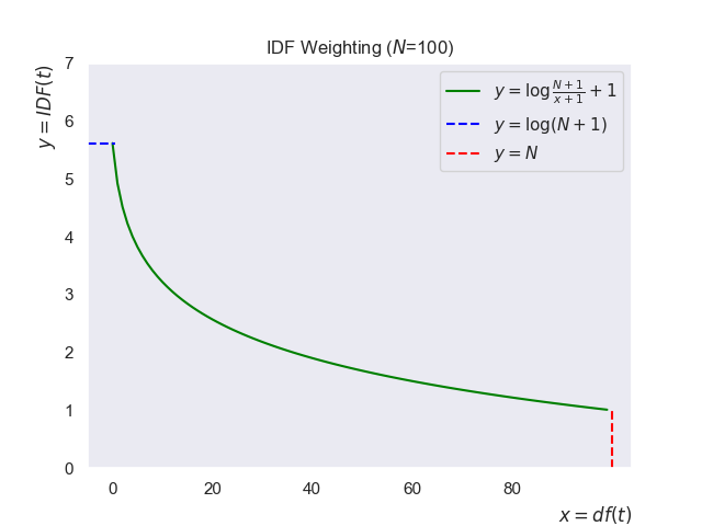
One of the most common IDF variants with smoothing is this:
\[IDF(t) = \log\frac{N+1}{df(t)+1} + 1\]This is also what scikit-learn uses when calculating IDF.
Here’s why the formula has all those extra +1s:
+1in the denominator: Without it, if a term never appears in the collection ($df(t) = 0$), you’d end up dividing by zero. The+1smooths this out so the math always works. You can think of it as “Even if the term is unseen, let’s pretend it appeared at least once.”+1in the numerator: If a term shows up in every document ($df(t) = N$), then $\log\frac{N}{N} = \log(1) = 0$. That would make the term’s weight vanish completely. By adding 1 to the numerator, those super-common terms still get a tiny but non-zero weight.+1outside the log: Even with smoothing inside the fraction, the log value can hover around zero or dip negative when terms are extremely common. Negative IDF values don’t make sense—TF-IDF weights should never imply “anti-importance.” Adding 1 outside guarantees that IDF stays positive, avoiding zeros or negatives.
Graphically:
With this smoothed IDF formula, our TF-IDF ranking function becomes:
\[f(q,d) = \sum_{i=1}^{n}\frac{c(t_i,d)(k+1)}{c(t_i,d)+k}(\log\frac{N+1}{df(t)+1}+1)\]In Python:
import math


def tf(term: str, document: str, k: float = 1.2) -> float:
    """
    Calculate TF score using bounded transformation.
    """
    # Apply some basic text normalization: 1. punctuation handling 2. lowercasing
    doc_terms = document.replace(".", " ").lower().split()
    term_count = doc_terms.count(term.lower())
    score = term_count * (k + 1) / (term_count + k)

    return score


def idf(term: str, documents: list[str]) -> float:
    """
    Calculate Inverse Document Frequency (IDF) for a term.
    """
    N = len(documents)  # Total number of documents
    df_t = 0
    for doc in documents:
        # Apply some basic text normalization: 1. punctuation handling 2. lowercasing
        if term.lower() in doc.replace(".", " ").lower().split():
            df_t += 1
    score = math.log((N + 1) / (df_t + 1)) + 1

    return score


def tf_idf_ranking_function(
    query: str, document: str, documents: list[str], k: float = 1.2
) -> float:
    """
    Calculate TF-IDF score
    """
    query_terms = query.lower().split()
    score: float = 0.0
    for term in query_terms:
        tf_score = tf(term, document, k)
        idf_score = idf(term, documents)
        score += tf_score * idf_score

    return score
Let’s revisit the query “korea interest rate” and four documents:
- d1: The Bank of Korea is expected to lower its benchmark interest rate next month.
- d2: A lower interest rate will be welcomed by indebted households.
- d3: The interest rate charged on loans is often higher than the interest rate paid on deposits.
- d4: The interest rate remains unchanged, but many fear this interest rate keeps loans costly while others welcome a stable interest rate.
Using TF-IDF ranking function, the scores are:
| documents | $f(q,d)$ ($k$=1.2) |
|---|---|
| d1 | 3.92 |
| d2 | 2 |
| d3 | 2.75 |
| d4 | 3.14 |
The ranking now matches user intent so that d1 rises above d4 because it contains the rarer term “Korea”.
Limitation
The ranking models discussed so far are inherently biased toward long documents. A longer document has a statistically higher chance of matching query terms, even if the matches are coincidental and scattered throughout the text.
Let’s look at one more document:
- d5: In South Korea, the central bank’s decision on the interest rate is closely watched by both businesses and households. Rising interest rate levels have slowed consumer spending, while exporters in Korea argue that a stable interest rate is necessary to remain competitive. Many in Korea believe that future growth depends on how carefully the government manages the interest rate policy.
Notice how d5 is stuffed with the words Korea and interest rate.
TF-IDF would likely push this document to the very top, not because it’s the most relevant, but simply because it’s long and keeps repeating the keywords.
The scores are:
| documents | $f(q,d)$ ($k$=1.2) |
|---|---|
| d1 | 3.69 |
| d2 | 2 |
| d3 | 2.75 |
| d4 | 3.14 |
| d5 | 5.71 |
That’s where Document Length Normalization comes in.
Document Length Normalization
The last heuristic is that longer documents naturally contain more terms, and therefore match queries more often. To counter this, their scores are adjusted relative to the average document length. The goal is simple: balance the bias toward long documents. In short, don’t reward a document just for being long.
Penalizing long documents must be done carefully to avoid over-penalization since a document can be long either because:
- It’s verbose: Some texts are just wordy. They take a simple idea and wrap it in way too many words. In this case, penalization makes sense.
- It’s comprehensive: Other texts are long because they actually cover more ground (like a news archive that bundles many different stories). These shouldn’t be punished too harshly, because their length comes from offering more useful, distinct content.
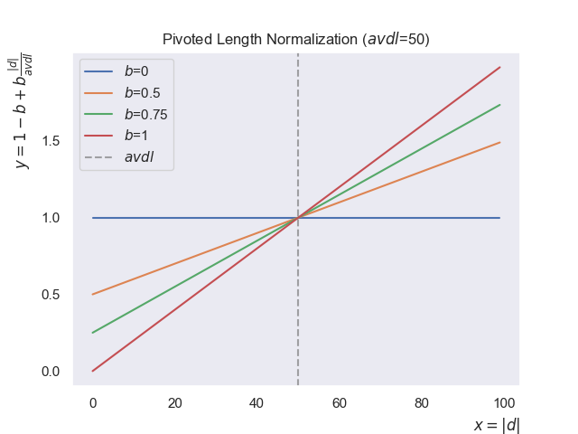
Pivoted Length Normalization
A robust solution to this problem is Pivoted Length Normalization. This method uses the average document length (avdl) of the entire collection as a “pivot” or reference point.
Here’s how it works in practice:
- Documents with a length equal to the
avdlreceive no penalty or reward (normalizer = 1). - Documents longer than the
avdlare penalized. - Documents shorter than the
avdlare rewarded.
The formula for the pivoted normalizer is:
\[normalizer = 1 - b + b \frac{|d|}{avdl}\]Where:
- $|d|$ is the length of the document (number of terms).
- $avdl$ is the average document length across the whole collection.
- $b$ is a tuning parameter between 0 and 1.
- If $b$ = 0, the normalizer is always 1, and no length normalization occurs.
- As $b$ increases towards 1, the penalty for long documents and the reward for short documents become more aggressive.
So where does this normalizer actually get applied?
In BM25, it slides into the denominator of the TF term. Here’s the BM25 TF function:
\[TF'(t,d) = \frac{c(t,d)(k+1)}{c(t,d)+k(1-b+b\frac{|d|}{avdl})}\]Finally, we arrive at the BM25 (Okapi) ranking function by integrating all three heuristics—TF Transformation, IDF Weighting, and Pivoted Length Normalization:
\[f(q,d) = \sum_{i=1}^{n}\frac{c(t_i,d)(k+1)}{c(t_i,d)+k(1-b+b\frac{|d|}{avdl})}(\log\frac{N+1}{df(t)+1}+1)\]Where:
- $k$ is the term frequency saturation parameter
- $b$ is the document-length normalization weight (0–1)
In Python:
import math


def tf_with_normalizer(term: str, document: str, k: float = 1.2, normalizer: float = 1.0) -> float:
    """
    Calculate TF score for a term using BM25 with document length normalization.
    """
    # Apply some basic text normalization: 1. punctuation handling 2. lowercasing
    doc_terms = document.replace(".", " ").lower().split()
    term_count = doc_terms.count(term.lower())
    score = term_count * (k + 1) / (term_count + k * normalizer)

    return score


def idf(term: str, documents: list[str]) -> float:
    """
    Calculate Inverse Document Frequency (IDF) for a term.
    """
    N = len(documents)  # Total number of documents
    df_t = 0
    for doc in documents:
        # Apply some basic text normalization: 1. punctuation handling 2. lowercasing
        if term.lower() in doc.replace(".", " ").lower().split():
            df_t += 1
    score = math.log((N + 1) / (df_t + 1)) + 1

    return score


def document_length_normalization(document: str, documents: list[str], b: float = 0.75) -> float:
    """
    Calculate document length normalization factor.
    """
    # Calculate average document length
    total_length = sum(len(doc.split()) for doc in documents)
    avdl = total_length / len(documents)
    doc_length = len(document.split())
    normalizer = 1 - b + b * (doc_length / avdl)

    return normalizer


def bm25_ranking_function(
    query: str, document: str, documents: list[str], k: float = 1.2, b: float = 0.75
) -> float:
    """
    Calculate BM25 score for a document given a query.

    Args:
        query: The query string.
        document: The document string.
        documents: The list of all documents. (collection)
        k: The term frequency saturation parameter.
        b: The length normalization parameter.
    """
    terms = query.lower().split()
    normalizer = document_length_normalization(document, documents, b)
    score: float = 0.0
    for term in terms:
        tf_score = tf_with_normalizer(term, document, k, normalizer)
        idf_score = idf(term, documents)
        score += tf_score * idf_score

    return score
Using the BM25 ranking function, the scores for our example become more acceptable:
| documents | $f(q,d)$ ($k$=1.2, $b$=0.75) |
|---|---|
| d1 | 4.46 |
| d2 | 2.63 |
| d3 | 3.04 |
| d4 | 3.23 |
| d5 | 4.34 |
What happens here is that even though d5 is long and loaded with repeated mentions of Korea and interest rate, it doesn’t unfairly dominate the ranking anymore.
Conclusion
BM25 is the backbone for many retrieval systems because it’s simple, fast, and surprisingly effective. But here’s one clear limitation: BM25 doesn’t actually understand context. It sees words, counts them, and scores documents based on math, not semantics.
Take these two documents:
- d1: The Bank of Korea is expected to lower its benchmark interest rate next month.
- d6: The interest in street dance across Korea has grown at such a fast rate.
And the query: “korea interest rate”
From BM25’s perspective, both documents look almost identical.
The same words appear, with the same frequency, so the scores end up nearly the same.
But to a human, the difference is obvious: d1 is clearly more relevant than d6.
That’s why modern search engines rarely rely on BM25 alone. Here are some techniques often used to address BM25’s limitations:
- Relevance feedback: learning from user clicks or pseudo-relevance feedback.
- Semantic embeddings: capturing meaning rather than just word overlap.
- Learning to Rank (LTR): training a machine learning model that combines multiple signals (BM25 scores, embeddings, click data, etc.) to optimize search result ordering.