
Langauge Models for Information Retrieval
In information retrieval (henceforth IR), the language modeling approach is a form of probabilistic retrieval. Unlike traditional probabilistic methods, which explicitly estimate the probability that a document is relevant to a query, the language modeling approach takes a different perspective. Instead of modeling relevance directly, it builds a probabilistic language model for each document and ranks documents based on the probability of the model generating the query.
The intuition is as follows. When someone seeks information, they have an implicit picture of the kinds of documents that they are looking for and the words those documents are likely to contain. Based on these imaginary documents and their representative terms, they choose search terms and send a query to a search engine, expecting the system to return those documents. The language modeling approach inverts this process. Given a document, it asks: “how likely is it that this document’s model would generate the given query?”
First, let’s review what the probabilistic modeling approach is in IR.
Probabilistic Modeling Approach
Probabilistic approaches to IR model ranking as an estimation problem. That is, given a query $q$ and a document $d$, we aim to estimate the probability that the document is relevant:
\[f(d,q) = P(R=1 \mid d,q), R \in {\{0,1\}}\]Where $R$ is a binary random variable indicating relevance.
Okapi BM25 is a non-binary model of the probabilistic model family.
The key question is: how do we realize this idea?
One intuitive approach is to use click-through logs as implicit relevance feedback. Suppose we have implicit relevance judgments mined from user clicks:
| $q$ | $d$ | $R$ |
|---|---|---|
| $q_1$ | $d_1$ | 1 |
| $q_1$ | $d_2$ | 0 |
| $q_1$ | $d_3$ | 0 |
| $q_1$ | $d_1$ | 1 |
| $q_1$ | $d_2$ | 0 |
| $q_1$ | $d_3$ | 1 |
| $q_2$ | $d_2$ | 1 |
| $q_2$ | $d_3$ | 0 |
For query $q_1$, we can estimate relevance for documents $d1$, $d2$, $d3$ by computing the fraction of exposures that resulted in a click: $p(R \mid d,q) = \frac{count(q,d,R=1)}{count(q,d)}$.
This yields:
- $P(R=1 \mid d_1,q_1) = 2/2 = 1$
- $P(R=1 \mid d_2,q_1) = 0/2 = 0$
- $P(R=1 \mid d_3,q_1) = 1/2 = 0.5$
So the ranking for $q_1$ would be $d_1 > d_3 > d_2$.
A clear limitation of this approach is that we have no data from which to estimate relevance if a document has never been shown before or if a query has never appeared. In practice, most queries are rare and most documents get little or no interaction.
The language modeling approach provides a different realization of probabilistic IR. Rather than estimating $P(R=1 \mid d,q)$, it reframes the problem as estimating how likely the document would generate the query:
\[P(q \mid d, R=1)\]In practice, it builds a probabilistic language model $M_d$ from each document $d$, and ranks documents based on the probability of the model generating the query:
\[P(q \mid M_d)\]This approach directly tackles the question in the intro: “how likely is it that this document’s model would generate the given query?”.
Let’s briefly go over what language models are and how they are constructed.
Language Models
A language model is a function that puts a probability measure over strings drawn from some vocabulary [An Introduction to Information Retrieval]. In the IR setting, these strings can be thought of as sequences of words or terms.
While often used interchangeably, it is useful to clarify three commonly used concepts:
- words: natural language units as written or spoken.
- terms: normalized tokens that an IR system indexes and matches.
- tokens: implementation-level units produced by a tokenizer, purely technical.
One of the simplest language models is a finite automaton, or simply a state machine, consisting of just a single node that generates terms based on a single probability distribution.
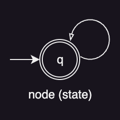
Because all terms are drawn independently from this distribution, the probabilities must sum to 1:
\[\sum_{t \in V}P(t)=1\]Where:
- $t$: term
- $V$: vocabulary
Since this model has no memory, each term is generated independently of the previous one. To compute the probability of a sequence, we simply multiply the term probabilities.
For example, here’s a partial specification of the term probabilities:
| $t$ | $P(t)$ |
|---|---|
| the | 0.2 |
| a | 0.1 |
| chocolate | 0.03 |
| milkshake | 0.02 |
| … | … |
Using this table, the probability of generating a string “chocolate milkshake” is:
\[P(\text{chocolate milkshake}) = P(\text{chocolate}) \times P(\text{milkshake}) = 0.03 \times 0.02 = 0.0006\]Such a model is often called “generative” because it can stochastically produce sequences of terms. A formal generative model would include a stop probability to decide whether to stop or to loop around and then produce another word. For example, if $P(\text{STOP}) = 0.2$, then $P(\text{chocolate milkshake}) = (0.03 \times 0.02) \times (0.8 \times 0.2) = 0.000096$. But in IR this factor cancels out when comparing models and does not affect ranking. Therefore, we omit to include stop probability in the IR context.
One use case of language models is association analysis, where we identify terms that are semantically related to a given seed word. Suppose we want to find words related to “vitamin”. We can build a topic language model $P_{topic}$ from documents containing that term:
| $t$ | $P_{topic}(t)$ |
|---|---|
| the | 0.04 |
| is | 0.03 |
| a | 0.01 |
| vitamin | 0.005 |
| nutrition | 0.004 |
Here, common terms like “the”, “is”, and “a” dominate the distribution, but they are not informative. To discount such common terms, we can compare the topic model against a background model constructed from a broad corpus:
| $t$ | $P_{background}(t)$ |
|---|---|
| the | 0.04 |
| is | 0.03 |
| a | 0.02 |
| vitamin | 0.00002 |
| nutrition | 0.00001 |
By taking the ratio $\frac{P_{topic}(t)}{P_{background}(t)}$, we highlight terms that are unusually frequent in the topic:
| $t$ | $P_{topic}(t)$ | $P_{background}(t)$ | $\frac{P_{topic}(t)}{P_{background}(t)}$ |
|---|---|---|---|
| nutrition | 0.004 | 0.00001 | 40 |
| vitamin | 0.005 | 0.00002 | 25 |
| the | 0.04 | 0.04 | 1 |
| is | 0.03 | 0.03 | 1 |
| a | 0.01 | 0.02 | 0.5 |
From this result, we can see which terms are common to both models and which are disproportionately frequent in the topic model. In particular, “nutrition” stands out as much more characteristic of the topic than generic words such as “the” or “is”, making it more likely to be semantically related to “vitamin”.
Unigram Language Model
The language models introduced so far belong to the simplest class called unigram language models. In a unigram model, the order of words does not matter. Because it treats a document as merely a collection of terms, it is often referred to as a “bag of words” approach. The model ignores all contextual dependencies and assumes that every term occurs independently:
\[P_{\text{uni}}(t_1 t_2 t_3)=P(t_1)P(t_2)P(t_3)\]There are more complex language models. For example, a bigram language model conditions each term on the term immediately preceding it:
\[P_{\text{bi}}(t_1 t_2 t_3)=P(t_1)P(t_2 \mid t_1)P(t_3 \mid t_2)\]More complex language models include trigram models and even grammar-based models that capture deeper structure in language. These richer models can be helpful in tasks such as:
- speech recognition
- spelling correction
- machine translation
All of these tasks depend on how likely a term is given the context that surrounds it.
In contrast, most language-modeling work in IR relies on unigram models as IR rarely depends on sentence structure. For determining what a document is about, unigram models are often sufficient. Unigram models are also computationally more efficient to estimate and apply than higher-order models. This efficiency makes them a good fit for large-scale IR systems, where speed and scalability are critical.
Maximum Likelihood Estimation
To estimate $P(q \mid M_d)$, we typically use maximum likelihood estimation (MLE). Under MLE, the probability of a term in a document is simply its frequency divided by the total number of tokens in that document:
\[{P}_{MLE}(t \mid M_d)=\frac{tf_{t,d}}{L_d}\]Where:
- $tf_{t,d}$ is the (raw) term frequency of term $t$ in document $d$
- $L_d$ is the number of tokens in document $d$
With MLE and the unigram assumption, the probability of producing the query $q$ from the document language model $M_d$ becomes:
\[\hat{P}(q \mid M_d) = \prod_{t \in q}\hat{P}_{MLE}(t \mid M_d) = \prod_{t \in q}\frac{tf_{t,d}}{L_d}\]Where $\hat{P}$ is the estimated probability.
Suppose a document $d$ contains 100 tokens ($L_d=100$), and we observe the following term frequencies:
| $t$ | $tf_{t,d}$ |
|---|---|
| chocolate | 10 |
| milkshake | 8 |
| … | … |
The corresponding MLE probabilities are:
| $t$ | $\frac{tf_{t,d}}{L_d}$ |
|---|---|
| chocolate | 10/100 |
| milkshake | 8/100 |
| … | … |
So, the probability of generating the query “chocolate milkshake” from $M_d$ is:
\[\hat{P}(\text{chocolate milkshake} \mid M_d) = \hat{P}_{MLE}(\text{chocolate} \mid M_d) \times \hat{P}_{MLE}(\text{milkshake} \mid M_d) = \frac{10}{100} \times \frac{8}{100} = 0.008\]Now that we know what language models are and how to estimate $P(q \mid M_d)$, we can move on to applying these ideas to the ranking problem. For simplicity, we will omit the estimator symbol $\hat{}$ on top of $P$ in the rest of the discussion.
Query Likelihood Model
The query likelihood model (often abbreviated as QLM) is the original and basic method for using language models in IR. The core assumption is that a user has some ideal or “prototype” document in mind and generates a query using terms that appear in that document. Whether users literally behave this way is debatable, but the intuition holds. That is, people tend to choose query terms they believe are representative and discriminative for the documents they want.
In QLM, we construct a language model $M_d$ for each document $d$ in the collection. Our goal is to rank documents by $P(d \mid q)$. This probability represents how likely it is that document $d$ is relevant to query $q$. Using Bayes’ rule:
\[P(d \mid q) = \frac{P(q \mid d)P(d)}{P(q)}\]Since $P(q)$ does not vary across documents, it can be ignored for ranking. The prior $P(d)$ is also commonly assumed to be uniform, so it can likewise be dropped. This leaves:
\[P(d \mid q) \propto P(q \mid d)\]In other words, we rank documents by the likelihood that the document’s language model would generate the query. Retrieval becomes a query-generation problem: the higher the likelihood, the more relevant the document.
The most common way to do this is using the unigram language model with MLE:
\[P(q \mid M_d) = \prod_{t \in V}P_{ML}(t \mid M_d)\]This assumes that each term in the query is generated independently, so we multiply their probabilities. Different ways of estimating $P(t \mid M_d)$ lead to different retrieval functions, and MLE is the simplest one.
In practice we can think of QLM as a three step process:
- Infer a LM for each document.
- Estimate $P(q \mid M_{d_{i}})$, the probability of generating the query according to each of these document models.
- Rank the documents according to these probabilities.
Here’s an example. Suppose the query is “chocolate milkshake”, and we have two documents, $d1$ and $d2$. By inferencing the document LMs for both documents, we get:
| $t$ | the | a | chocolate | milkshake | … |
|---|---|---|---|---|---|
| $M_{d_1}$ | 0.2 | 0.1 | 0.03 | 0.02 | … |
| $M_{d_2}$ | 0.2 | 0.1 | 0.02 | 0.01 | … |
Using MLE, we can then compute the term probabilities in each document model:
- $P(\text{chocolcate milkshake}\mid M_{d_1})=0.03 \times 0.02=0.0006$
- $P(\text{chocolcate milkshake}\mid M_{d_2})=0.02 \times 0.01=0.0002$
Since $0.0006 \gt 0.0002$, we rank $d_1 \gt d_2$.
In practice, multiplying many small probabilities leads to floating-point underflow, where the outcome is so small that it can no longer be represented by the computer. To avoid this, sums of log probabilities is often used:
\[f(q,d) = \log{P(q \mid M_d)} = \sum_{i=1}^{n}\log{P(t_i \mid M_d)} = \sum_{t \in V}tf_{t,q}\log{P(t \mid M_d)}\]Where $tf_{t,q}$ is the (raw) term frequency of term $t$ in query $q$.
This transformation preserves ranking, since the logarithm is a monotonic function.
A major limitation of the basic query likelihood approach arises when a query term does not appear in a document. Under MLE, it gives $P(t \mid M_d)=0$, making the entire query likelihood zero. Even in log space, MLE assigns $\log{P(t \mid M_d)}=-\infty$, making the entire query likelihood $-\infty$. The result is an overly strict conjunctive (AND-style) retrieval where a document contributes only if it contains every query term. In addition, even observed terms are poorly estimated under MLE. Rare terms tend to be overestimated because their single occurrence may be due to chance. The solution is smoothing.
Smoothing
Smoothing is a way to discount non-zero probabilities and to give some probability mass to unseen terms. The general approach is to assign a non-zero probability to unseen terms based on the whole collection. That is:
\[P(t \mid d) = \begin{cases} P(t \mid M_d), & \text{if } tf_{t,d} > 0,\\ \alpha_{d}\,P(t \mid M_c), & \text{otherwise} \end{cases}\]Where:
- $\alpha_d$ is a smoothing factor of document $d$ for unseen terms.
- $M_c$ is a language model built from the entire collection.
For a term that doesn’t appear in document $d$, we fall back on the collection probability:
\[P(t \mid M_c)=\frac{cf_t}{T}\]Where:
- $cf_t$ is the raw count of the term in the collection
- $T$ is the raw size (number of terms) of the entire collection
With this idea, the ranking function becomes:
\[\begin{aligned} \log P(q \mid d) &= \sum_{t \in V}tf_{t,q}\log{P(t \mid M_d)} \\ &= \sum_{t \in V, tf_{t,d}>0}tf_{t,q}\log{P(t \mid M_d)} + \sum_{t \in V, tf_{t,d}=0}tf_{t,q}\log\alpha_{d}{P(t \mid M_c)} \\ &= \sum_{t \in V, tf_{t,d}>0}tf_{t,q}\log{P(t \mid M_d)} + (\sum_{t \in V}tf_{t,q}\log\alpha_{d}{P(t \mid M_c)} - \sum_{t \in V, tf_{t,d}>0}tf_{t,q}\log\alpha_{d}{P(t \mid M_c)}) \\ &= \sum_{t \in V, tf_{t,d}>0}tf_{t,q}\log{\frac{P(t \mid M_d)}{\alpha_{d}{P(t \mid M_c)}}} + \vert q \vert \log\alpha_{d} + \sum_{t \in V}tf_{t,q}\log{P(t \mid M_c)} \end{aligned}\]We can make this equation simpler by removing the $\sum_{t \in V}tf_{t,q}\log{P(t \mid M_c)}$ part as it’s going to be the same for every document and doesn’t affect ranking. So:
\[\log P(q \mid d) = \sum_{t \in V, tf_{t,d}>0}tf_{t,q}\log{\frac{P(t \mid M_d)}{\alpha_{d}{P(t \mid M_c)}}} + \vert q \vert \log\alpha_{d}\]This transformation automatically provides two benefits:
- More efficient computation as scoring is only based on matched query terms
- The effects of TF-IDF weighting and document length normalization:
- $P(t \mid M_d)$ behaves like TF.
- $\frac{1}{P(t \mid M_c)}$ behaves like IDF.
- $\vert q \vert \log\alpha_{d}$ acts like document length normalization, because longer documents usually need a smaller $\alpha_{d}$.
A takeaway here is that the role of smoothing is not only to avoid zero probabilities. The smoothing of terms actually implements major parts of the term weighting component.
Next up are the specific smoothing methods that have been shown to perform well in IR experiments:
- Jelinek-Mercer smoothing
- Dirichilet Prior smoothing
Jelinek-Mercer Smoothing
Jelinek-Mercer smoothing, also referred to as as linear interpolation smoothing, is the simpleest smoothing method. The idea is to mix two sources of information. One comes from the document itself and the other comes from the whole collection:
\[P(t \mid d)=(1-\lambda)P(t \mid M_d) + \lambda P(t \mid M_c)\]Where $\lambda$ is a smoothing factor that controls the extent of smoothing ($0 < \lambda < 1$). A large value of $\lambda$ means more smoothing.
A useful property is that $\lambda$ doesn’t have to be a fixed constant and you can make it depend on the query length. For example:
- For short queries: use a small $\lambda$
- For long queries: use a larger $\lambda$
If we substitute the JM formula into our scoring function, we get:
\[\begin{aligned} f_{JM}(q \mid d) &= \sum_{t \in V, tf_{t,d}>0}tf_{t,q}\log{\frac{(1-\lambda)P(t \mid M_d) + \lambda P(t \mid M_c)}{\lambda{P(t \mid M_c)}}} + \vert q \vert \log\lambda \\ &= \sum_{t \in V, tf_{t,d}>0}tf_{t,q}\log{\frac{(1-\lambda)P(t \mid M_d) + \lambda P(t \mid M_c)}{\lambda{P(t \mid M_c)}}} + \vert q \vert \log\lambda\\ &= \sum_{t \in V, tf_{t,d}>0}tf_{t,q}\log{(1+\frac{1-\lambda}{\lambda}\frac{tf_{t,d}}{L_d P(t \mid M_c)})} + \vert q \vert \log\lambda \end{aligned}\]Since, $\vert q \vert \log\lambda$ is the same for every document, we can drop it for ranking purposes. So:
\[f_{JM}(q \mid d) = \sum_{t \in V, tf_{t,d}>0}tf_{t,q}\log{(1+\frac{1-\lambda}{\lambda}\frac{tf_{t,d}}{L_d P(t \mid M_c)})}\]Below are the interpretations of some parts in this equation:
- $\lambda$ plays the role of the smoothing factor (similar to $\alpha_d$).
- $tf_{t,q}$ acts like TF weighting.
- $\frac{1}{P(t \mid M_c)}$ acts like IDF weighting.
- $\frac{1}{L_d}$ provides document length normalization.
So even though this looks like a language-modeling formula, it ends up recreating a lot of the same behavior as classic TF-IDF ranking.
Here’s an example. Suppose our collection has two documents:
- $d_1$: “Here is a recipe for a classic, creamy chocolate milkshake”
- $d_2$: “Dark chocolate is a little bitter but very delicious”
We’ll use basic unigram MLEs for both the documents and the whole collection, and we’ll set $\lambda = 0.5$. Now take the query: “chocolate milkshake”
Then:
\[f(q \mid d_1) = \log\left(1 + \frac{1 - 0.5}{0.5} \cdot \frac{1}{10 \cdot \frac{2}{19}}\right) + \log\left(1 + \frac{1 - 0.5}{0.5} \cdot \frac{1}{10 \cdot \frac{1}{19}}\right) = 1.73\] \[f(q \mid d_2) = \log\left(1 + \frac{1 - 0.5}{0.5} \cdot \frac{1}{9 \cdot \frac{2}{19}}\right) + \log\left(1 + \frac{1 - 0.5}{0.5} \cdot \frac{0}{9 \cdot \frac{1}{19}}\right) = 0.72\]Only $d_1$ contains “milkshake”, so it gets a strong boost in score. The ranking ends up as $d_1 \gt d_2$. Notice that even though $d_2$ does not contain “milkshake” at all it still receives a non zero score because smoothing gives it some probability mass.
Dirichilet Prior Smoothing
Dirichilet Prior smoothing, also called as Bayesian smoothing, takes a different angle from Jelinek–Mercer. Instead of mixing two models with a fixed weight, it treats the collection language model as a prior and then updates it using evidence from the document.
The formula is:
\[P(t \mid d)=\frac{L_d}{L_d+\alpha}P(t \mid M_d) + \frac{\alpha}{L_d+\alpha} P(t \mid M_c)= \frac{tf_{t,d} + \alpha P(t \mid M_c)}{L_d + \alpha}\]Where
- $L_d$ is the number of terms in document $d$
- $\alpha$ is a smoothing factor ($\alpha \in [0, +\infty)$). A large value of $\alpha$ means more smoothing.
This equation has an intuitive interpretation:
- If a document is short, $L_d$ is small, so the model leans more toward the collection (more smoothing).
- If a document is long, $L_d$ dominates, so the model trusts the document more (less smoothing).
Using this expression, the scoring function becomes:
\[\begin{aligned} f_{DIR}(q \mid d) &= \sum_{t \in V, tf_{t,d}>0}tf_{t,q}\log{\frac{\frac{tf_{w,d}+\alpha P(t \mid M_c)}{L_d+\alpha}}{\frac{\alpha P(t \mid M_c)}{L_d+\alpha}}} + \vert q \vert \log\frac{\alpha}{L_d+\alpha} \\ &= \sum_{t \in V, tf_{t,d}>0}tf_{t,q}\log{(1+\frac{tf_{t,d}}{\alpha P(t \mid M_c)})}+\vert q \vert \log\frac{\alpha}{L_d+\alpha} \end{aligned}\]Just like JM smoothing, this method naturally gives tf-idf weighting and document length normalization. Specifically:
- $tf_{t,q}$ -> TF weighting
- $\frac{1}{P(t \mid M_c)}$ -> IDF weighting
-
$ q \log\frac{\alpha}{L_d+\alpha}$ -> document length normalization
A key difference from JM smoothing is that the effective weight ($\alpha_d$) becomes $\frac{\alpha}{L_d+\alpha}$ instead of the fixed linear coefficient $\lambda$. This means the model automatically smooths short documents more and long documents less, which makes the interpolation adaptive rather than fixed.
Other Language Modeling Approaches
Up to this point, we’ve focused on a single perspective that is query likelihood. However, there are other language modeling approaches worth mentioning.
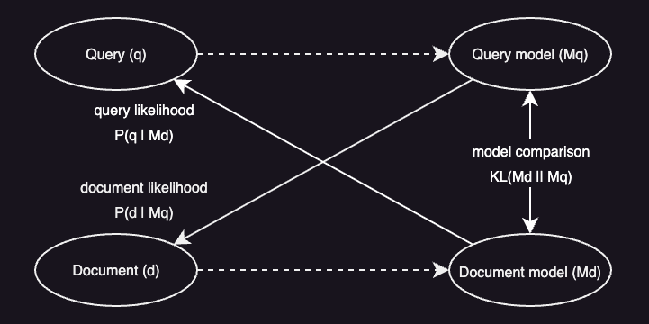
Document Likelihood
Document likelihood looks at how likely a query language model $M_q$ is to generate a document $d$:
\[P(d \mid M_q)\]In theory, it’s a symmetric idea of query likelihood. In practice, though, it’s not well suited for direct document ranking. Queries are typically short, providing too little data to estimate a reliable query model. As a result, the model becomes unstable and performs poorly when used on its own.
The upside is that this approach naturally supports relevance feedback. We can expand the query model with terms from documents judged relevant, making it easier to refine the query representation.
Model Comparison
Another approach builds a language model for both the document and the query, then measures how different the two models are. One common way to quantify this difference (or “risk”) of returning document $d$ for query $q$ is the Kullback-Leibler (KL) divergence:
\[R(d;q)=KL(M_d \mid\mid M_q)=\sum_{t \in V}(P \mid M_q)\log{\frac{P(t \mid M_q)}{P(t \mid M_d)}}\]The greater the divergence, the less the document model resembles the query model, and the poorer the match.
A limitation of KL-based scoring is that the scores aren’t comparable across different queries. This is fine for ad hoc retrieval, where we only care about ranking documents within a single query. But in applications like topic tracking, where we need one global threshold to decide whether a document belongs to a topic across many queries, the lack of score comparability becomes a significant drawback.
LM Similarities Supported by Elasticsearch
Elasticsearch, a widely used search engine built on top of Lucene, provides built-in language-model-based similarity modules that support both Jelinek Mercer smoothing and Dirichlet Prior smoothing.
Below is a minimal example (tested on Elasticsearch 8.19) showing how to set up an index that applies different scoring strategies to identical text.
The index declares three text fields, each tied to a different similarity:
PUT /my-index
{
  "settings": {
    "index": {
      "similarity": {
        "jm_similarity": {
          "type": "LMJelinekMercer",
          "lambda": "0.1"
        },
        "dirichlet_similarity": {
          "type": "LMDirichlet",
          "mu": 2000
        }
      }
    }
  },
  "mappings": {
    "properties": {
      "bm25": {
        "type": "text"
      },
      "jm": {
        "type": "text",
        "similarity": "jm_similarity"
      },
      "dirichlet": {
        "type": "text",
        "similarity": "dirichlet_similarity"
      }
    }
  }
}
bm25uses the default BM25 similarity.jmuses Jelinek–Mercer smoothing.dirichletuses Dirichlet prior smoothing.
By indexing the same content into three fields, you can directly compare how each method ranks the same documents for the same query.
Add sample documents:
PUT /my-index/_doc/1
{
  "bm25": "foo bar baz",
  "jm": "foo bar baz",
  "dirichlet": "foo bar baz"
}

PUT /my-index/_doc/2
{
  "bm25": "Lorem ipsum dolor sit amet",
  "jm": "Lorem ipsum dolor sit amet",
  "dirichlet": "Lorem ipsum dolor sit amet"
}
This query searches the dirichlet field for the term “foo”:
GET my-index/_search
{
    "query": {
        "match": {
          "dirichlet": "foo"
        }
    }
}
Document 1 matches, but the key point is the scoring behavior. Even though the underlying text is identical across fields, each similarity computes a different score:
| BM25 | JM | Dirichlet | |
|---|---|---|---|
| score | 0.7721133 | 2.6741486 | 0.00074859645 |
Conclusion
According to Ponte and Croft (1998), the language modeling approach outperformed their baseline tf-idf based term weighting approach. They pointed out that the language modeling approach gives a new way to score how well a query matches a document. The idea is that by using a probabilistic model of language, we can assign better weights to terms and, as a result, improve retrieval performance. The major issue is estimation of the document model, such as choices of how to smooth it effectively [An Introduction to Information Retrieval].
Despite many advances in probabilistic IR, BM25 still remains competitive and often hard to beat. In practice, BM25 and query likelihood models tend to perform similarly. However, BM25 has a clear practical advantage because it lets us directly and intuitively control how term frequency and document length affect the final score.