
Understanding PageRank
Query-dependent ranking models such as TF-IDF and BM25 are not sufficient for web search because they mainly measure how closely the terms in a query match the content of a page. In other words, they do not indicate whether a page is trustworthy, authoritative, or important.
PageRank, created by Google’s co-founders including Larry Page, addresses this limitation by analyzing the link structure of the web. It ranks web pages by counting the number and quality of links to a page to estimate the page’s importance. The fundamental heuristic is that a page is likely to be important if many other important pages link to it. This sounds a bit circular, and it is. We will see how PageRank solves that problem in this post.
Since PageRank is a link analysis algorithm, let’s briefly go over link analysis first.
Link Analysis in Web Search
Link analysis in web search is inspired by citation analysis, a field that studies the influence of academic papers by examining how they cite one another, also known as bibliometrics. A citation can be viewed as a signal that one paper considers another useful or authoritative.
Hyperlinks work in a similar way. When one webpage links to another, that link can be interpreted as a signal that the linked page is trustworthy, authoritative, or important. However, there are some significant differences between academic publications and web pages.
Academic publications are carefully reviewed and are generally similar in purpose, structure, and quality. Web pages, on the other hand, are much easier to create, so they vary widely in quality, length, purpose, and popularity. They can also be created in large numbers to manipulate link-based signals or search rankings (a.k.a. link spam). Therefore, simply counting links is not enough.
A more reliable approach is to consider not only how many links a page receives but also the quality of the pages providing those links. This idea is sometimes described as indirect citation. In other words, a link from an important page should carry more weight than a link from a less important one.
Another well-known link-analysis algorithm used in web search is HITS. In HITS, each page receives two scores: an authority score, which measures how valuable the page is as a source of information, and a hub score, which measures how effectively the page links to authoritative sources.
Random Surfer Model
The random surfer model provides an intuitive way to understand how PageRank works. In this model, we imagine a hypothetical surfer on the internet who randomly clicks on links.
Consider a collection of four wep pages: A, B, C, and D. The link structure of these pages are as follows:
- Page A does not link to any other page.
- Page B links to page A: (B -> A)
- Page C links to pages A and B: (C -> A), (C -> B)
- Page D links to pages A, B, and C: (D -> A), (D -> B), (D -> C)
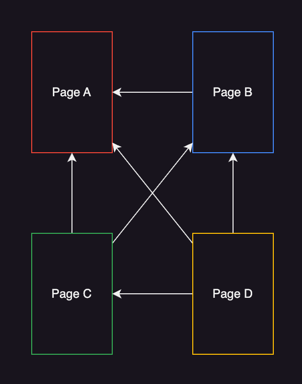
The random surfer starts with a web page at random, and then randomly clicks links to follow. For example, if the surfer is on page C, they randomly choose between page A and page B. If they choose page B, they then follow its only outgoing link to page A.
Here, the PageRank value of a page is the probability the random surfer will land on that page at any given time. Therefore, a page with many incoming links (sometimes called backlinks or inlinks) would receive a higher PageRank because the surfer is more likely to reach it. For example, page A receives links from B, C, and D, while page C receives a link only from D. We can intuitively expect page A to have a higher PageRank than page C.
This model naturally captures the idea of indirect links as well. That is, a link from an important page carries more weight because the surfer is more likely to visit that page and then follow one of its outgoing links. For example, page B links to page A, and page B itself receives links from C and D. As a result, page B passes some of its importance on to page A, increasing A’s PageRank.
This model can also be viewed as a Markov chain. Each webpage represents a state, and each link represents a possible transition to another state. The probability of the surfer’s next move depends only on the current page, not on the pages visited before it. For example, if the surfer is currently on page C, the next page will be either A or B, each with probability 1/2, regardless of how the surfer arrived at C.
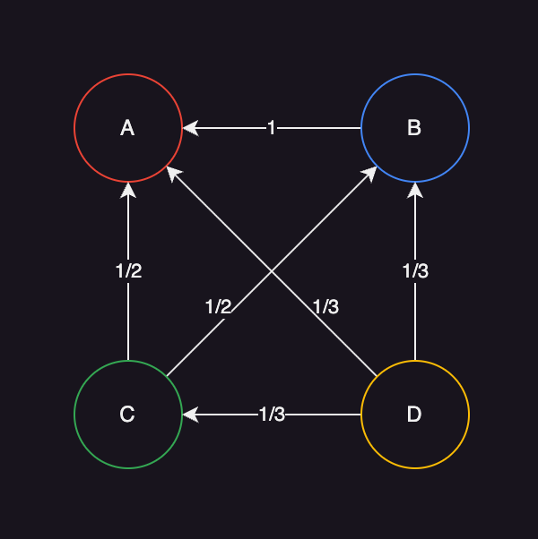
Algorithm
Letting $PR(p)$ be the PageRank of a given page $p$, here’s how we define $PR(p)$ in its simplest form:
\[PR(p_j)=\sum_{p_i \in M{(p_{j})}}\frac{PR(p_i)}{L(p_i)}\]Where:
- $p_{1},p_{2},\cdots,p_{N}$: the pages under consideration
- $M{(p_{j})}$: the set of pages that link to page $p_j$
- $L(p_i)$: the number of outgoing links on page $p_i$
For example, to calculate the PageRank of page A, we add the PageRank contributions from every page that links to it: B, C, and D. Each of these pages divides its PageRank equally among its outgoing links. Therefore:
\[PR(A)=\frac{PR(B)}{L(B)}+\frac{PR(C)}{L(C)}+\frac{PR(D)}{L(D)}=\frac{PR(B)}{1}+\frac{PR(C)}{2}+\frac{PR(D)}{3}\]To make the algorithm more robust, standard preprocessing rules apply:
- Links from a page to itself are ignored to prevent pages from boosting their own importance.
- Duplicate links from one page to the same page count only once to prevent artificial inflation.
However, this simplified model has two important problems:
- Rank sinks (spider traps): If a group of pages links only to each other, the surfer can become trapped in a closed loop and never reach the rest of the web. Once the surfer enters it, the group may absorb an increasing amount of probability mass, causing the PageRank of all pages outside that loop may eventually drop to zero.
- Dangling pages (dead ends): If a page has no outgoing links, the surfer has nowhere to go. The PageRank received by that page cannot be passed on to other pages, so some rank is lost during each iteration.
The first problem is addressed by introducing a damping factor $d$. The second requires special handling of dangling pages, typically by treating each one as if it linked uniformly to every page in the collection.
Damping factor
The damping factor $d$ represents the probability that the surfer continues following links instead of jumping to a random page.
At each step, the random surfer follows a randomly chosen outgoing link with probability $d$, or jumps (teleports) to any random page in the collection with probability $1 − d$. With the damping factor $d$, the PageRank equation becomes:
\[PR(p_{j})=\frac{1-d}{N}+d\sum_{p_{i}\in M(p_{j})}\frac{PR(p_{i})}{L(p_{i})}\]Where:
- $p_{1},p_{2},\cdots,p_{N}$: the pages under consideration
- $M{(p_{j})}$: the set of pages that link to page $p_j$
- $L(p_i)$: the number of outgoing links on page $p_i$
- $N$: the total number of pages
- $d$: the damping factor (usually set around 0.85)
The first term $\frac{1-d}{N}$ represents the probability of random jumping to $p_{j}$, while the second represents the probability of reaching $p_{j}$ by following links. This random jump, known as teleportation, ensures that the surfer can never be permanently trapped.
Handling dangling pages
Once the surfer reaches a dangling page, there is no link to follow. To prevent probability mass from being lost, we treat a dangling page as though it links to every page in the collection with equal probability. So, the transition probability from a dangling page to any page in the collection is $\frac{1}{N}$.
If we construct the transition matrix $\mathcal{M}$ where \(\mathcal{M}_{i,j}\) is the transition probability from $p_{i}$ to $p_{j}$, then:
\[\mathcal{M}_{i,j} = \begin{cases} \dfrac{1}{L(p_i)}, & \text{if } p_i \text{ links to } p_j, \\[6pt] \dfrac{1}{N}, & \text{if } p_i \text{ is a dangling page}, \\[6pt] 0, & \text{otherwise}. \end{cases}\]Because every row represents a complete probability distribution over destination pages, the rows sum to 1:
\[\sum_{j=1}^{N}\mathcal{M}_{i,j}=1\]This guarantees that $\mathcal{M}$ is a row-stochastic matrix.
Notice that a dangling page is treated as if it links to every page, including itself. This may seem to conflict with one of the preprocessing rules, that self-links should be ignored. However, these rules apply to different situations. The rule against self-links removes real HTML links to stop website owners from artificially boosting their rank. But the dangling-page rule is a mathematical fallback to keep the calculation from breaking when it hits a dead end.
Finally, recall that the restricted sum $\sum_{p_i \in M(p_j)}$ in our earlier equation only accounted for pages with direct outgoing links to $p_j$. It would therefore omit the redistributed probability mass from dangling pages. Since $\mathcal{M}_{i,j}=0$ whenever a non-dangling page $p_i$ does not link to $p_j$, we can safely replace the restricted sum with a sum over all $N$ pages:
\[PR(p_{j})={\frac{1-d}{N}}+d\sum_{i=1}^{N}\mathcal{M_{i,j}}{PR(p_{i})}\]This equation accounts for both normal link transitions, teleportation, and the redistributed probability mass from dangling pages.
Computation: Iterative method
Because PageRank is defined recursively, it can be computed using an iterative method.
We begin by assigning an initial PageRank value to every page. The initial probability distribution is usually chosen to be uniform across all $N$ pages in the collection. So, at iteration $t=0$:
\[PR_0(p_j)=\frac{1}{N}\]At each iteration, the PageRank of every page is updated using the PageRank values from the previous iteration:
\[PR_{t+1}(p_{j})={\frac{1-d}{N}}+d\sum_{i=1}^{N}\mathcal{M_{i,j}}{PR_{t}(p_{i})}\]Since PageRank is a normalized probability distribution, the sum of all PageRanks across the collection equals 1:
\[\sum_{i=1}^{N} PR(p_i) = 1\]This property allows us to rewrite the constant term $\frac{1-d}{N}$ and combine the entire expression into a single summation:
\[\begin{aligned} PR_{t+1}(p_j) &= \frac{1-d}{N} + d \sum_{i=1}^{N} \mathcal{M}_{i,j} PR_{t}(p_i) \\ &= \frac{1-d}{N} \cdot (1) + d \sum_{i=1}^{N} \mathcal{M}_{i,j} PR_{t}(p_i) \\ &= \frac{1-d}{N} \left( \sum_{i=1}^{N} PR_{t}(p_i) \right) + d \sum_{i=1}^{N} \mathcal{M}_{i,j} PR_{t}(p_i) \\ &= \sum_{i=1}^{N} \frac{1-d}{N} PR_{t}(p_i) + \sum_{i=1}^{N} d \mathcal{M}_{i,j} PR_{t}(p_i) \\ &= \sum_{i=1}^{N} \left( \frac{1-d}{N} + d \mathcal{M}_{i,j} \right) PR_{t}(p_i) \end{aligned}\]This expression inside the parentheses \(\left( \frac{1-d}{N} + d \mathcal{M}_{i,j} \right)\) defines the entry $G_{i,j}$ of the so-called Google matrix $G$:
\[G_{i,j} = \frac{1-d}{N} + d \mathcal{M}_{i,j}\]Here, $G_{i,j}$ represents the overall transition probability of a random surfer moving from page $p_i$ to page $p_j$:
So, the iterative update can also be written as:
\[PR_{t+1}(p_j) = \sum_{i=1}^{N} G_{i,j} PR_{t}(p_i)\]There is one such PageRank equation for every page $p_j$, giving a system of $N$ equations. We can express all $N$ equations at once by defining the pagerank vector at iteration $t$ as:
\[\mathbf {R_t} ={\begin{bmatrix}PR_{t}(p_{1})\\PR_{t}(p_{2})\\\vdots \\PR_{t}(p_{N})\end{bmatrix}}\]Therefore, the solution of the $N$ equations is:
\[\mathbf{R_{t+1}}=\begin{bmatrix}\frac{1-d}{N}\\\frac{1-d}{N}\\\vdots\\\frac{1-d}{N}\end{bmatrix}+d\begin{bmatrix}\mathcal{M}_{1,1}&\mathcal{M}_{2,1}&\cdots&\mathcal{M}_{N,1}\\\mathcal{M}_{1,2}&\mathcal{M}_{2,2}&\cdots&\mathcal{M}_{N,2}\\\vdots&\vdots&\ddots&\vdots\\\mathcal{M}_{1,N}&\mathcal{M}_{2,N}&\cdots&\mathcal{M}_{N,N}\end{bmatrix}\mathbf{R_{t}}\]Recall that the transition matrix $\mathcal{M}$ is defined as:
\[\mathcal{M} = \begin{bmatrix} \mathcal{M}_{1,1} & \mathcal{M}_{1,2} & \cdots & \mathcal{M}_{1,N} \\ \mathcal{M}_{2,1} & \mathcal{M}_{2,2} & \cdots & \mathcal{M}_{2,N} \\ \vdots & \vdots & \ddots & \vdots \\ \mathcal{M}_{N,1} & \mathcal{M}_{N,2} & \cdots & \mathcal{M}_{N,N} \end{bmatrix}\]where \(\mathcal{M}_{i,j}\) is the transition probability from $p_{i}$ to $p_{j}$.
Since the matrix in the equation above is the transpose of $\mathcal{M}$, the equation becomes:
\[\mathbf{R_{t+1}}=\frac{1-d}{N}\mathbf{1}+d\mathcal{M}^{\intercal}\mathbf{R_{t}}\]where $\mathbf{1}$ is the $N$-dimensional vector whose entries are all equal to $1$.
In some literature, the transition matrix uses the opposite convention: $\mathcal{M}_{i,j}$ is the probability of moving from $p_j$ to $p_i$. In that case, the PageRank equation is written without a transpose, for example, $\mathbf{R}=\frac{1-d}{N}\mathbf{1}+d\mathcal{M}\mathbf{R}$. So, don’t be confused.
Equivalently:
\[\mathbf{R_{t+1}}=G^{\intercal}\mathbf{R_{t}}\]Repeatedly applying this matrix–vector multiplication is known as the power method.
As $t \to \infty$, this iterative process converges to stationary PageRank vector R. That is:
\[PR_{t+1}(p_j) = PR_t(p_j) = PR(p_j)\]Once equilibrium is reached, we can drop the time index $t$:
\[\mathbf{R}=G^{\intercal}\mathbf{R}\]Thus, $\mathbf{R}$ is a right eigenvector of $G^{\intercal}$ with eigenvalue 1. Each entry of $\mathbf{R}$ represents the long-run probability that a random surfer is on the corresponding page.
In practice, the algorithm does not run for infinitely many iterations. Instead, it stops when two consecutive PageRank vectors are sufficiently close. For example:
\[\vert\mathbf{R}_{t+1}-\mathbf{R}_t\vert < \epsilon\]where $\epsilon$ is a convergence tolerance.
Example
Let’s return to our previous example which consists of four wep pages: A, B, C, and D. Since the collection contains four pages, $N=4$.
We will compute the PageRank vector after one iteration, denoted by $\mathbf{R_1}$:
\[\mathbf{R_1}=\frac{1-d}{N}\mathbf{1}+d\mathcal{M}^{\intercal}\mathbf{R_0}\]We first define the transition matrix $\mathcal{M}$:
\[\mathcal{M} = \begin{pmatrix} \textcolor{#EA4335}{\frac{1}{4}} & \textcolor{#EA4335}{\frac{1}{4}} & \textcolor{#EA4335}{\frac{1}{4}} & \textcolor{#EA4335}{\frac{1}{4}} \\ \textcolor{#4285F4}{1} & \textcolor{#4285F4}{0} & \textcolor{#4285F4}{0} & \textcolor{#4285F4}{0} \\ \textcolor{#34A853}{\frac{1}{2}} & \textcolor{#34A853}{\frac{1}{2}} & \textcolor{#34A853}{0} & \textcolor{#34A853}{0} \\ \textcolor{#FBBC05}{\frac{1}{3}} & \textcolor{#FBBC05}{\frac{1}{3}} & \textcolor{#FBBC05}{\frac{1}{3}} & \textcolor{#FBBC05}{0} \end{pmatrix}\]Page A has no outgoing links, so it’s a dangling page. To handle this, we treat Page A as if it links to every page, including itself, with equal probability. Therefore, every entry in the first row is $\textcolor{#E57373}{\frac{1}{4}}$.
With this dangling-page rule applied, the Markov chain graph looks:
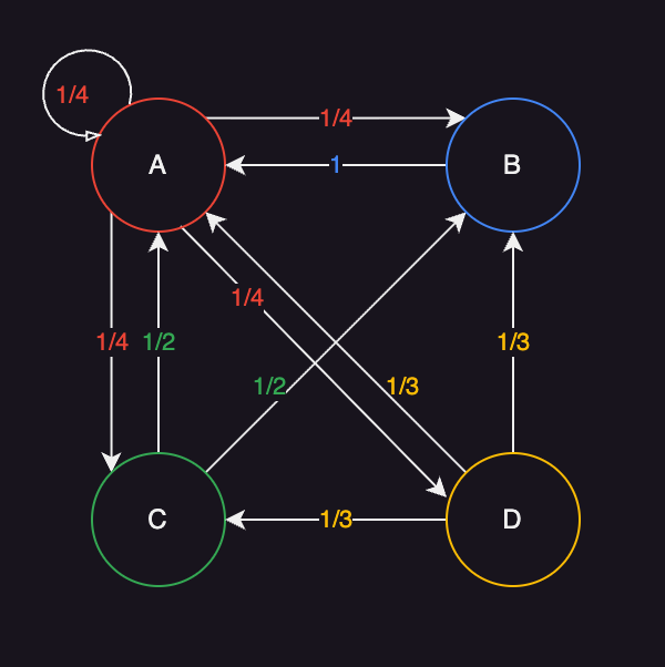
Since the initial probability distribution is usually chosen to be uniform across all $N$ pages in the collection:
\[\mathbf{R_0}=\begin{pmatrix} \frac{1}{4} \\ \frac{1}{4} \\ \frac{1}{4} \\ \frac{1}{4} \end{pmatrix}\]Using a damping factor of $d=0.85$, we can compute the $\mathbf{R_1}$ as follows:
\[\begin{aligned} R_1 &= \frac{1 - 0.85}{4} \begin{pmatrix} 1 \\ 1 \\ 1 \\ 1 \end{pmatrix} + 0.85 \begin{pmatrix} \textcolor{#EA4335}{\frac{1}{4}} & \textcolor{#EA4335}{\frac{1}{4}} & \textcolor{#EA4335}{\frac{1}{4}} & \textcolor{#EA4335}{\frac{1}{4}} \\ \textcolor{#4285F4}{1} & \textcolor{#4285F4}{0} & \textcolor{#4285F4}{0} & \textcolor{#4285F4}{0} \\ \textcolor{#34A853}{\frac{1}{2}} & \textcolor{#34A853}{\frac{1}{2}} & \textcolor{#34A853}{0} & \textcolor{#34A853}{0} \\ \textcolor{#FBBC05}{\frac{1}{3}} & \textcolor{#FBBC05}{\frac{1}{3}} & \textcolor{#FBBC05}{\frac{1}{3}} & \textcolor{#FBBC05}{0} \end{pmatrix}^T \begin{pmatrix} \frac{1}{4} \\ \frac{1}{4} \\ \frac{1}{4} \\ \frac{1}{4} \end{pmatrix} \\ &= \frac{1 - 0.85}{4} \begin{pmatrix} 1 \\ 1 \\ 1 \\ 1 \end{pmatrix} + 0.85 \begin{pmatrix} \textcolor{#EA4335}{\frac{1}{4}} & \textcolor{#4285F4}{1} & \textcolor{#34A853}{\frac{1}{2}} & \textcolor{#FBBC05}{\frac{1}{3}} \\ \textcolor{#EA4335}{\frac{1}{4}} & \textcolor{#4285F4}{0} & \textcolor{#34A853}{\frac{1}{2}} & \textcolor{#FBBC05}{\frac{1}{3}} \\ \textcolor{#EA4335}{\frac{1}{4}} & \textcolor{#4285F4}{0} & \textcolor{#34A853}{0} & \textcolor{#FBBC05}{\frac{1}{3}} \\ \textcolor{#EA4335}{\frac{1}{4}} & \textcolor{#4285F4}{0} & \textcolor{#34A853}{0} & \textcolor{#FBBC05}{0} \end{pmatrix} \begin{pmatrix} \frac{1}{4} \\ \frac{1}{4} \\ \frac{1}{4} \\ \frac{1}{4} \end{pmatrix} \\ &= \begin{pmatrix} 0.0375 \\ 0.0375 \\ 0.0375 \\ 0.0375 \end{pmatrix} + 0.85 \begin{pmatrix} 0.5208 \\ 0.2708 \\ 0.1458 \\ 0.0625 \end{pmatrix} \\ &= \begin{pmatrix} 0.0375 \\ 0.0375 \\ 0.0375 \\ 0.0375 \end{pmatrix} + \begin{pmatrix} 0.4427 \\ 0.2302 \\ 0.1240 \\ 0.0531 \end{pmatrix} \\ &= \begin{pmatrix} 0.4802 \\ 0.2677 \\ 0.1615 \\ 0.0906 \end{pmatrix} \end{aligned}\]Therefore, after one iteration, the PageRank scores are:
\[R_1 = \begin{pmatrix} 0.4802 \\ 0.2677 \\ 0.1615 \\ 0.0906 \end{pmatrix}\]As expected, the probabilities sum to 1:
\[0.4802+0.2677+0.1615+0.0906=1\]We can continue applying the same update rule until the PageRank vector converges.
Implementation
The following code calculates PageRank with the transition matrix and damping factor:
import numpy as np


def calculate_pagerank(
    M: np.ndarray,
    d: float = 0.85,
    max_t: int = 10,
    epsilon: float = 1e-8,
) -> np.ndarray:
    """Compute PageRank scores using the power iteration method.

    Args:
        M: Transition matrix.
        d: Damping factor.
        max_t: Maximum number of iterations.
        epsilon: Convergence tolerance.

    Returns:
        The PageRank score vector.
    """
    M_T = M.T  # Transpose the transition matrix
    N = len(M_T)  # Number of pages
    R = np.full(N, 1.0 / N)  # Initialize the rank vector with equal probabilities
    teleport = (1.0 - d) / N  # Teleportation vector

    for t in range(max_t):
        next_R = teleport + d * (M_T @ R)
        # Check for convergence
        if np.abs(next_R - R).sum() < epsilon:
            R = next_R
            break
        R = next_R

    return R
After computing the next rank vector, the function measures the total absolute difference between the old and new vectors.
If this difference is smaller than epsilon, the scores are considered to have converged.
We can now use this function to calculate the PageRank scores for our example. The following code runs the algorithm for 10 iterations and prints the resulting scores:
# Define the transition matrix M
M = np.array(
    [
        [1 / 4, 1 / 4, 1 / 4, 1 / 4],  # From page A
        [1, 0, 0, 0],  # From page B
        [1 / 2, 1 / 2, 0, 0],  # From page C
        [1 / 3, 1 / 3, 1 / 3, 0],  # From page D
    ]
)
pagerank_scores = calculate_pagerank(M=M, d=0.85, max_t=10)
print("PageRank scores:")
pages = ["A", "B", "C", "D"]
final_ranks = dict(zip(pages, pagerank_scores))
for page, score in final_ranks.items():
    print(f"Page {page}: {score:.4f}")
The output is:
PageRank scores:
Page A: 0.4514
Page B: 0.2440
Page C: 0.1712
Page D: 0.1334
As expected, Page A receives the highest PageRank score, while Page D receives the lowest.
To see how the algorithm approaches these values, we can examine the PageRank vector after each iteration:
| $t$ | Page A | Page B | Page C | Page D |
|---|---|---|---|---|
| 0 | 0.25000000 | 0.25000000 | 0.25000000 | 0.25000000 |
| 1 | 0.48020833 | 0.26770833 | 0.16145833 | 0.09062500 |
| 2 | 0.46139323 | 0.23384115 | 0.16522135 | 0.13954427 |
| 3 | 0.44406765 | 0.24530268 | 0.17508360 | 0.13554606 |
| 4 | 0.45318690 | 0.24467963 | 0.17026909 | 0.13186438 |
| 5 | 0.45150584 | 0.24352816 | 0.17116379 | 0.13380222 |
| 6 | 0.45109916 | 0.24410023 | 0.17135562 | 0.13344499 |
| 7 | 0.45147932 | 0.24399412 | 0.17116799 | 0.13335857 |
| 8 | 0.45136568 | 0.24397068 | 0.17122428 | 0.13343936 |
| 9 | 0.45136842 | 0.24399335 | 0.17122302 | 0.13341521 |
| 10 | 0.45138089 | 0.24398655 | 0.17121677 | 0.13341579 |
At the beginning, the scores change substantially because the initial uniform distribution does not reflect the link structure. The values then go up and down around their limiting values, but the size of these changes decreases with each iteration. This shows how power iteration converges: by repeatedly applying the PageRank update, the rank vector gradually moves toward a stable distribution of the random-surfing process.
Limitations
PageRank measures popularity, not relevance or quality. A popular page may have a high PageRank but still be unrelated to the search query. For this reason, PageRank must be combined with content-based or query-dependent ranking methods.
PageRank can favor established sites. Pages that already have many links are more likely to receive high scores and gain even more visibility. This makes it harder for new or less-known pages to rank well, even when they contain useful information.
PageRank can still be manipulated. Website owners can create artificial links to increase a page’s score. For example, groups of websites can link to one another or to a target page.
Conclusion
PageRank is arguably the foundational algorithm responsible for Google’s early success in web search. Since then, it has also been adapted across many other fields. For example, it has been applied to rank scientific papers, and evaluate teams or players using sports match data.
One nice thing about PageRank is that it scales surprisingly well. In the original paper, Google’s founders reported that PageRank took about 52 iterations to converge on a graph with 322 million links, while graph about half that size took around 45 iterations. Based on this, they suggested that the number of iterations grows roughly like $\log{n}$, where $n$ is the size of the graph.