
Relevance Feedback and Query Expansion
The problem of a pure keyword matching approach is that the systems can’t handle synonymy issue. For example, you might search for “python” meaning the programming language, not the snake. And a query for “sea” may fail to match documents that use “ocean” instead.
Two common ways to address this problem are relevance feedback and query expansion. In relevance feedback, the system adjusts the query based on the documents that seem relevant in the first round of retrieval. In query expansion, a query is expanded or reformulated to match other semantically similar terms.
Relevance Feedback
Relevance feedback is used to improve both recall and precision. The main idea is simple: use feedback from users to refine the query.
The process is typically as follows:
- The user issues a query.
- The system returns an initial set of results.
- The user judges relevance of returned documents.
- The system updates the query based on the user feedback.
- The system returns a revised set of results.
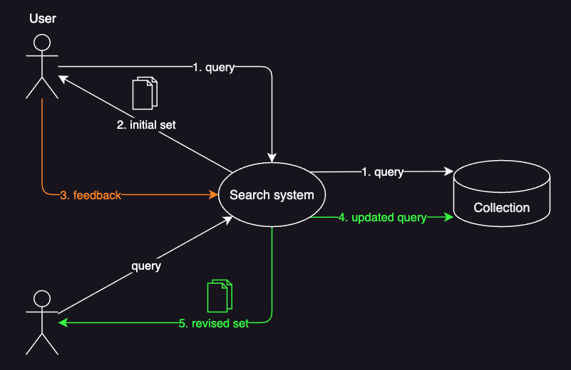
Based on how step 3 is handled, there are three main types of relevance feedback:
- Explicit relevance feedback
- Implicit relevance feedback
- Pseudo relevance feedback (also called blind or automatic relevance feedback)
Explicit Relevance Feedback
In explicit relevance feedback, or just relevance feedback, users are asked to judge returned documents. In practice, though, this approach is often limited because most users do not want to spend extra effort during search. This is especially true when they have no strong incentive to provide that feedback. It also becomes less practical when the result set is large, since judging many documents takes time.
Even so, explicit relevance feedback can still be useful in laboratory or experimental settings, where users may be motivated to provide relevance judgments.
Implicit Relevance Feedback
In implicit, or indirect, relevance feedback, the system uses user behavior logs such as clickthrough as relevance signals. For example, documents clicked for a query may be treated as relevant, while documents that are not clicked may be treated as less relevant. A higher number of clicks may also be interpreted as a stronger relevance signal.
This is probably the most common approach in real retrieval systems, because it does not ask users to provide explicit judgments. It is also easier to collect at scale in systems with many users and large amounts of interaction data.
One limitation is that these signals are not always reliable. A click does not always mean a document is relevant: it may be accidental, or even malicious.
Ranking advertisements for a search query in a web search engine is a closely related application of this idea.
Pseudo Relevance Feedback
In pseudo relevance feedback, also called blind or automatic relevance feedback, the top-k documents in the initial results are assumed to be relevant.
So, unlike explicit or implicit feedback, this method does not require any user input.
Because it makes that assumption automatically, it is generally less reliable than other forms of relevance feedback.
For example, if the query is “john wick” and the top-k documents are mostly about Keanu Reeves, the updated query may drift toward documents about Keanu Reeves rather than the film itself.
One useful application of this method is association anaylsis. For example, we can build a topic language model and compare it with the collection language model to extract terms that are strongly related to a given query. These related terms can then be added to the original query. This is a form of query expansion, which we will discuss later in this post.
The Rocchio Algorithm
The Rocchio algorithm is the most effective classic relevance feedback method in vector space model. It is used in step 4, where the system updates the query based on user feedback.
The basic idea is to build a new query vector $\vec{q}$ that is closer to relevant documents and farther from nonrelevant ones. In other words, we want a query vector that increases similarity to relevant documents while decreasing similarity to nonrelevant documents.
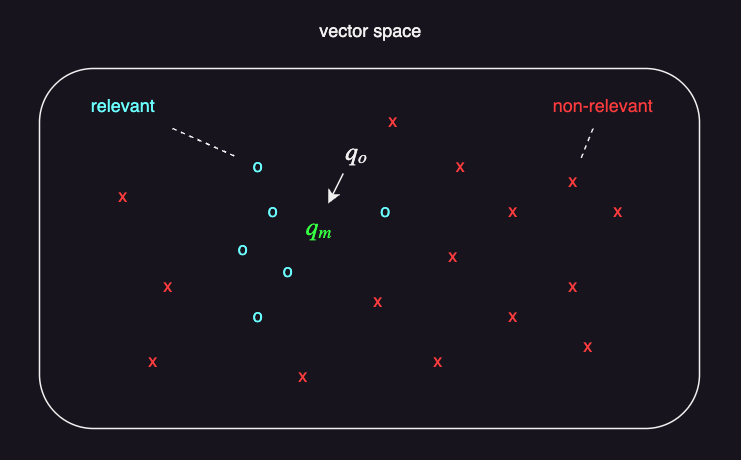
To do so, we need some knowledge of what documents are relevant (positive) and nonrelevant (negative). This is where relevance feedback comes in. Once we have the knowledge, we can move the initial query vector toward the centroid of the relevant documents and away from the centroid of the nonrelevant documents.
The formula is:
\[\vec{q}_m=\alpha\vec{q}_o + \beta\frac{1}{\vert D_r \vert}\sum_{\vec{d}_j \in D_r}\vec{d}_j - \gamma\frac{1}{\vert D_{nr} \vert}\sum_{\vec{d}_j \in D_{nr}}\vec{d}_j\]Where:
- $\vec{q_m}$: the modified (new) vector
- $\vec{q_o}$: the original query vector
- $D_r$: the set of known relevant documents
- $D_{nr}$: the set of known nonrelevant documents
- $\alpha$: the original query weight
- $\beta$: the related documents weight
- $\gamma$: the nonrelated documents weight
- $\frac{1}{\vert D_r \vert}\sum_{\vec{d}_j \in D_r}\vec{d}_j$: the centroid (vector) of positive examples
- \(\frac{1}{\vert D_{nr} \vert}\sum_{\vec{d}_j \in D_{nr}}\vec{d}_j\): the centroid (vector) of negative examples
As the formula shows, three parameters ($\alpha$, $\beta$, $\gamma$) control how much weight we give to the original query, the relevant documents, and the nonrelevant documents. For example, if we have enough judged documents to trust the feedback, we may want to use higher values for $\beta$ and $\gamma$.
In practice, $\alpha$ is usually kept relatively high to preserve the importance of the original query vector. This also helps avoid overfitting when the number of feedback samples is small. Meanwhile, $\gamma$ is often kept small, or even set to 0. This is because nonrelevant documents are not always clustered together, so they can push the query in many different directions. Therefore, reasonable values might be something like:
- $\alpha$ = 1
- $\beta$ = 0.5
- $\gamma$ = 0.1
Here’s an example.
Suppose the query $\vec{q}$ is hybrid search, and the system returns four documents:
| Document | Text |
|---|---|
| D1 | a successful search system |
| D2 | hybrid search in Elasticsearch |
| D3 | hybrid search combines keyword search and semantic search |
| D4 | hybrid engine can reduce fuel consumption |
The user judges the second and third documents as relevant, and the fourth document as nonrelevant:
| Document | Text | Feedback |
|---|---|---|
| D1 | a successful search system | |
| D2 | hybrid search in Elasticsearch | O |
| D3 | hybrid search combines keyword search and semantic search | O |
| D4 | hybrid engine can reduce fuel consumption | X |
We first need to define a consistent term order for the vector dimensions. If we list the unique terms from the query and the four documents in alphabetical order, we get:
('a', 'and', 'can', 'combines', 'consumption', 'Elasticsearch', 'engine', 'fuel', 'hybrid', 'in', 'keyword', 'reduce', 'search', 'semantic', 'successful', 'system')
So this is a 16-dimensional vector space.
Assume the search engine uses term frequency, but not length normalization or IDF. Then each document can be represented as follows:
| Document | Text | Feedback | Vector |
|---|---|---|---|
| D1 | a successful search system | $(1, 0, 0, 0, 0, 0, 0, 0, 0, 0, 0, 0, 1, 0, 1, 1)$ | |
| D2 | hybrid search in Elasticsearch | O | $(0, 0, 0, 0, 0, 1, 0, 0, 1, 1, 0, 0, 1, 0, 0, 0)$ |
| D3 | hybrid search combines keyword search and semantic search | O | $(0, 1, 0, 1, 0, 0, 0, 0, 1, 0, 1, 0, 3, 1, 0, 0)$ |
| D4 | hybrid engine can reduce fuel consumption | X | $(0, 0, 1, 0, 1, 0, 1, 1, 1, 0, 0, 1, 0, 0, 0, 0)$ |
The query $\vec{q}$ in the same vector space is:
\[\vec{q} = (0, 0, 0, 0, 0, 0, 0, 0, 1, 0, 0, 0, 1, 0, 0, 0)\]Assume the system uses Rocchio relevance feedback with $\alpha = 1$, $\beta = 1$, and $\gamma = 0$. Then the modified query becomes:
\[\vec{q}_m = \vec{q}_0 + \frac{1}{2} (\vec{d}_2 + \vec{d}_3) - \frac{0}{1} (\vec{d}_4)\]Since $\gamma = 0$, the nonrelevant document $\vec{d}_4$ is ignored.
So the final modified query vector $\vec{q}_m$ is:
\[\begin{aligned} \vec{q}_m &= (0, 0, 0, 0, 0, 0, 0, 0, 1, 0, 0, 0, 1, 0, 0, 0) \\ &+ \frac{1}{2} \big( (0, 0, 0, 0, 0, 1, 0, 0, 1, 1, 0, 0, 1, 0, 0, 0) + (0, 1, 0, 1, 0, 0, 0, 0, 1, 0, 1, 0, 3, 1, 0, 0) \big) \\ &= (0, 0, 0, 0, 0, 0, 0, 0, 1, 0, 0, 0, 1, 0, 0, 0) + \frac{1}{2} (0, 1, 0, 1, 0, 1, 0, 0, 2, 1, 1, 0, 4, 1, 0, 0) \\ &= (0, 0, 0, 0, 0, 0, 0, 0, 1, 0, 0, 0, 1, 0, 0, 0) + (0, 0.5, 0, 0.5, 0, 0.5, 0, 0, 1, 0.5, 0.5, 0, 2, 0.5, 0, 0) \\ &= (0, 0.5, 0, 0.5, 0, 0.5, 0, 0, 2, 0.5, 0.5, 0, 3, 0.5, 0, 0) \end{aligned}\]In a more readable format:
\[\vec{q}_m = \begin{pmatrix} \text{a}: 0 \\ \text{and}: 0.5 \\ \text{can}: 0 \\ \text{combines}: 0.5 \\ \text{consumption}: 0 \\ \text{Elasticsearch}: 0.5 \\ \text{engine}: 0 \\ \text{fuel}: 0 \\ \text{hybrid}: 2.0 \\ \text{in}: 0.5 \\ \text{keyword}: 0.5 \\ \text{reduce}: 0 \\ \text{search}: 3.0 \\ \text{semantic}: 0.5 \\ \text{successful}: 0 \\ \text{system}: 0 \end{pmatrix}\]One potential problem of this method is computational cost. After relevance feedback, the updated query vector may contain many terms from relevant documents. In our example, the original query has only 2 non-zero terms, but the updated query has 8.
In practice, we often truncate the modified vector and keep only the highest-weighted terms for efficiency.
In the modified query vector above, the top terms are search (3.0), hybrid (2.0), and then several terms with weight 0.5.
If we keep only the top 3 terms, the new query becomes roughly search hybrid Elasticsearch.
As the Rocchio algorithm works within a vector space model, it is not limited to text retrieval systems. It can be applied to any type of data that can be represented as vectors, including images, audio, and learned embeddings.
Demonstration
For this demonstration, I embedded a collection of images from Pixabay. I used openai/clip-vit-base-patch32 to generate the image embeddings, then reduced them to a 256-dimensional vector space.
The first image shows the initial results for the query “cat”:

Now suppose the user marks six images as relevant (blue boxes) and two cat food images as nonrelevant (red boxes):
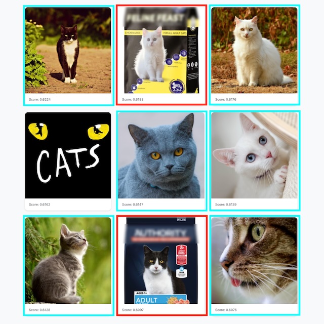
At this point, the system has useful information about which documents are relevant and which are nonrelevant for the query cat. Using this feedback, we can modify the query vector with the Rocchio algorithm.
The next image shows the revised results after updating the query vector with $\alpha=1$, $\beta=0.5$, and $\gamma=0.1$:
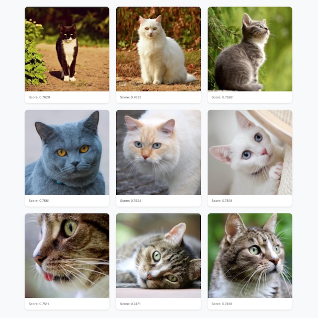
As you can see, the images explicitly marked as non-relevant no longer appear in the results, and more relevant images are shown instead.
However, increasing $\gamma$ can hurt the results. The next image shows the revised results when the query vector is updated with $\alpha=1$, $\beta=0.5$, and $\gamma=0.8$:

In this result set, nonrelevant images are mixed in with the cat images because the query is pulled too strongly by the negative examples.
For reference, here is the Rocchio implementation I used in this demonstration:
import numpy as np


def get_modified_query_vector(
    original_query_vector: np.ndarray,
    relevant_document_vectors: list[np.ndarray],
    nonrelevant_document_vectors: list[np.ndarray],
    alpha: float = 1.0,
    beta: float = 0.1,
    gamma: float = 0,
) -> np.ndarray:
    """
    Calculate the modified query vector using the Rocchio algorithm.

    Args:
        original_query_vector: The original query vector.
        relevant_document_vectors: List of vectors for relevant documents.
        nonrelevant_document_vectors: List of vectors for non-relevant documents.
        alpha: Weight for the original query vector.
        beta: Weight for the relevant document vectors.
        gamma: Weight for the non-relevant document vectors.

    Returns:
        The modified query vector.
    """
    # Calculate the mean vector of relevant documents
    if len(relevant_document_vectors) > 0:
        mean_relevant_vector = np.mean(relevant_document_vectors, axis=0)
    else:
        mean_relevant_vector = np.zeros_like(original_query_vector)

    # Calculate the mean vector of non-relevant documents
    if len(nonrelevant_document_vectors) > 0:
        mean_nonrelevant_vector = np.mean(nonrelevant_document_vectors, axis=0)
    else:
        mean_nonrelevant_vector = np.zeros_like(original_query_vector)

    # Apply the Rocchio formula
    modified_query_vector = (
        alpha * original_query_vector
        + beta * mean_relevant_vector
        - gamma * mean_nonrelevant_vector
    )

    return modified_query_vector
Constraints and Limitations
Relevance feedback alone may not be sufficient in certain conditions:
- Misspellings or typos. These are better handled with spelling correction.
- Cross-language information retrieval. For example, if you search for “global warming” in a collection of Korean documents that use the term “지구 온난화”, relevance feedback may not help if it only learns associations between English terms. This problem is usually handled with machine translation or cross-lingual semantic mapping.
- Synonymy. If you search for “laptop” but the documents use “notebook computer,” the query may miss relevant results. One way to handle this is query expansion using a predefined dictionary or thesaurus.
The Rocchio algorithm represents relevant documents with a single centroid, so it works best when those documents form a cluster. It may not work well when relevant documents are split into groups that use different vocabulary, such as “Burma” and “Myanmar.” (The country of Burma was renamed to Myanmar in 1989.)
Relevance feedback is also less useful in web search. Its main benefit is often improved recall, but most web search users do not care much about high recall. They are usually satisfied if the system returns a small number of highly relevant results.
Query Expansion
In relevance feedback, user feedback is used to modify the query vector. In query expansion, the original query is replaced with an alternative query or expanded with related terms. Like relevance feedback, query expansion is primarily used to improve recall.
There are two main ways to do this:
- Interactive query expansion: The system shows users related queries, and the user chooses one of them. This is often called query suggestion. For example, if a user searches for
apple, the interface might suggest queries such asapple storeorapple support. - Automatic query expansion: The system automatically adds synonyms or related terms to the query. For example, if a user searches for
Burma, the system may also search forMyanmar. In this case, the user may not even notice that the query has been expanded.
The main problem is how to generate these alternative or expanded queries.
The most common approach is to use some form of thesaurus.
That is, for each term t in the query, the system can expand the query with synonyms or related words for t taken from the thesaurus.
A thesaurus-based approach has the advantage that it does not require user feedback.
The entries in a thesaurus can be created manually or generated automatically.
Manual Thesaurus
In a manual thesaurus, developers or human editors manage sets of synonyms and alternative terms. This approach is especially useful in specialized domains, where term relationships need to be carefully curated. It can also be useful for fast-changing or trendy queries, where developers want to quickly add related terms that may not yet appear in a general thesaurus.
When building a thesaurus from scratch, developers can start from public or open-source thesauri. For example, the UMLS Metathesaurus is a useful resource for building search systems in the biomedical domain.
A simple yet practical way to build up a thesaurus is to use a document database like Elasticsearch. By leveraging an inverted index, each synonym can be looked up quickly, making it easy to retrieve the full synonym list from a query term.
For example, we can create a simple thesaurus index like this:
PUT thesaurus
{
  "mappings": {
    "properties": {
      "synonyms": {
        "type": "keyword"
      }
    }
  }
}
If you need to designate canonical terms for each set of synonyms, then you can add another field such as canonical_term:
PUT thesaurus
{
  "mappings": {
    "properties": {
      "synonyms": {
        "type": "keyword"
      },
      "canonical_term": {
        "type": "keyword"
      }
    }
  }
}
A canonical term is the preferred or normalized form of a synonym group. For example, you might want to treat “burma” as a synonym, but internally normalize it to “myanmar”.
You can add an entry to this thesaurus like this:
POST thesaurus/_doc
{
  "synonyms": [
    "burma",
    "myanmar"
  ]
}
Then, when a user searches for one term, you can look it up in the thesaurus and retrieve the full synonym group. For example, if the query contains “burma”, we can search for thesaurus entries that include that term:
GET thesaurus/_search
{
  "query": {
    "term": {
      "synonyms": "burma"
    }
  }
}
Response:
{
  ...,
  "hits": {
    ...,
    "hits": [
      {
        ...,
        "_source": {
          "synonyms": [
            "burma",
            "myanmar"
          ]
        }
      }
    ]
  }
}
Now the search system can expand the original query using the returned synonym set.
Automatic Thesaurus Generation
Because building a manual thesaurus is expensive, we can try to generate one automatically.
One approach is to use word co-occurrence statistics over a document collection. The idea is that words that co-occur in the same document or paragraph are likely to be semantically similar or related.
The simplest way to build a co-occurrence thesaurus is to compute term-term similarity. This approach starts with a term-document matrix $A$:
| $d_1$ | $d_2$ | $d_3$ | |
|---|---|---|---|
| $t_1$ | $A_{t_1,d_1}$ | $A_{t_1,d_2}$ | $A_{t_1,d_3}$ |
| $t_2$ | $A_{t_2,d_1}$ | $A_{t_2,d_2}$ | $A_{t_2,d_3}$ |
| $t_3$ | $A_{t_3,d_1}$ | $A_{t_3,d_2}$ | $A_{t_3,d_3}$ |
Each cell $A_{t,d}$ is a weight $w_{t,d}$ of term $t$ in document $d$. If we compute $C = AA^T$, then each entry $C_{u,v}$ measures how strongly terms $u$ and $v$ are related. The larger the value, the more related the two terms are.
Here’s a simple example. Suppose we have three documents:
- $d_1$ (about cars)
- $d_2$ (about cars)
- $d_2$ (about fruit)
And four terms:
- $t_1$: car
- $t_2$: automobile
- $t_3$: engine
- $t_4$: banana
Let the term-document matrix $A$ be:
| $d_1$ | $d_2$ | $d_3$ | |
|---|---|---|---|
| car | 1.0 | 0.8 | 0.0 |
| automobile | 0.9 | 1.0 | 0.0 |
| engine | 0.8 | 0.7 | 0.0 |
| banana | 0.0 | 0.0 | 1.0 |
Notice that “car”, “automobile”, and “engine” are strong in $d_1$ and $d_2$ while banana only appears in $d_3$.
By multipyling $A$ and $A^T$:
\[\begin{bmatrix} 1.0 & 0.8 & 0.0 \\ 0.9 & 1.0 & 0.0 \\ 0.8 & 0.7 & 0.0 \\ 0.0 & 0.0 & 1.0 \end{bmatrix} \times \begin{bmatrix} 1.0 & 0.9 & 0.8 & 0.0 \\ 0.8 & 1.0 & 0.7 & 0.0 \\ 0.0 & 0.0 & 0.0 & 1.0 \end{bmatrix} = \begin{bmatrix} 1.64 & 1.70 & 1.36 & 0.00 \\ 1.70 & 1.81 & 1.42 & 0.00 \\ 1.36 & 1.42 & 1.13 & 0.00 \\ 0.00 & 0.00 & 0.00 & 1.00 \end{bmatrix}\]we get the term-term matrix $C$:
| car | automobile | engine | banana | |
|---|---|---|---|---|
| car | 1.64 | 1.70 | 1.36 | 0.0 |
| automobile | 1.70 | 1.81 | 1.42 | 0.0 |
| engine | 1.36 | 1.42 | 1.13 | 0.0 |
| banana | 0.00 | 0.00 | 0.00 | 1.0 |
Each $C_{u,v}$ is just the dot product of the row for term $u$ and the row for term $v$:
\[C_{u,v} = \sum_{d}A_{u,d}A_{v,d}\]For example, the similarity between “car” and “engine” is:
\[\begin{aligned} C_{\text{car}, \text{engine}} &= [1.0, 0.8, 0.0] \cdot [0.8, 0.7, 0.0] \\ &= 1.0\cdot0.8 + 0.8\cdot0.7 + 0.0\cdot0.0 \\ &= 1.36 \end{aligned}\]So, the system can build entries like:
- car -> automobile, engine
- automobile -> car, engine
- banana -> (none of these)
Constraints and Limitations
A manual thesaurus is expensive to build and maintain. For domain-specific systems, a general thesaurus is often not enough, because it may not cover specialized vocabulary well. For example, in medical or legal search systems, specialized terminology and relationships must be covered as well.
A thesaurus generated automatically from co-occurrence statistics also has clear limits. It does not necessarily capture true synonyms. Instead, it captures words that have similar distributions across documents, such as “car” and “engine”. Its quality also depends heavily on the document collection. If the corpus is small, the statistics may be unreliable. If the corpus is biased toward a particular topic, the thesaurus will reflect that bias. For example, in a general-language corpus, likely neighbors of the term “virus” might be “pathogen”, “infection”, and “germ”. But if the corpus is heavily biased toward medicine and public health, virus may co-occur much more often with words like “vaccine”, “patient”, and “outbreak”. As a result, the generated thesaurus may rank those words highly.
Elasticsearch Support for Query Expansion
Elasticsearch, an open-source search and analytics engine, supports the significant_terms and significant_text aggregations.
These can be useful for discovering related terms automatically, at least to some extent.
These do not compute plain co-occurrence counts. Instead, they find terms that are unusually common in a foreground set compared with a background set:
- Foreground set: the search results matched by a query
- Background set: the index or indices from which the results were gathered
For example, the following query searches headlines for “health” and finds terms that are unusually common in the headline field of those results compared with the whole index:
GET news_categories/_search
{
  "size": 0,
  "query": {
    "match": {
      "headline": "health"
    }
  },
  "aggregations": {
    "keywords": {
      "significant_text": {
        "field": "headline"
      }
    }
  }
}
Response:
{
  ...
  "hits": {
    "total": {
      "value": 2349,
      "relation": "eq"
    },
    "max_score": null,
    "hits": []
  },
  "aggregations": {
    "keywords": {
      "doc_count": 2349,
      "bg_count": 628581,
      "buckets": [
        ...
        {
          "key": "care",
          "doc_count": 706,
          "score": 14.049006021392186,
          "bg_count": 3957
        },
        {
          "key": "mental",
          "doc_count": 270,
          "score": 6.105789285390884,
          "bg_count": 1335
        },
        {
          "key": "insurance",
          "doc_count": 85,
          "score": 1.3707596512376896,
          "bg_count": 585
        },
        ...
      ]
    }
  }
}
The results suggest that “care”, “mental”, and “insurance” are strongly associated with “health” in headlines.
Take “care” as an example.
It appears in the headline field of 3,957 documents in the full index, as shown by bg_count.
Of those, 706 appearances are in the 2,349 documents whose headlines matched “health”.
That means “care” is unusually common in the foreground set compared with the background set, so Elasticsearch considers it significant.
A user might then choose to add “care” to the query, for example to expand a search for “health” into something like “health care” or to otherwise improve recall.
(The demonstration uses the News Category Dataset by Rishabh Misra from Kaggle, licensed under CC BY 4.0.)
The query above is the simplest way to use the significant_text aggregation.
However, re-analyzing many matching documents requires a lot of time and memory.
For better performance, it is recommended using significant_text aggregation with a sampler, as shown below:
GET news_categories/_search
{
  "size": 0,
  "query": {
    "match": {
      "headline": "health"
    }
  },
  "aggregations": {
    "my_sample": {
      "sampler": {
        "shard_size": 100
      },
      "aggregations": {
        "keywords": {
          "significant_text": {
            "field": "headline"
          }
        }
      }
    }
  }
}
One advantage of this approach over raw co-occurrence is that it automatically suppresses globally common words. However, just like co-occurrence statistics, the selected terms are not necessarily similar or related terms.
Conclusion
For improving recall, relevance feedback is generally more effective than query expansion. That said, finding good values for the Rocchio weights, $\alpha$, $\beta$, and $\gamma$, is still a problem.
Query expansion, on the other hand, can hurt precision if it is used carelessly. However, it is easier for developers to understand than relevance feedback. Therefore, it is much more straightforward to implement, reason about, and debug.
References
- An Introduction to Information Retrieval by Christopher D. Manning, Prabhakar Raghavan, and Hinrich Schütze
- Text Retrieval and Search Engines by University of Illinois Urbana-Champaign
- Rocchio algorithm - Wikipedia
- Significant terms aggregation - Elasticsearch
- Significant text aggregation - Elasticsearch