
Introduction to Learning to Rank with Python
A formal definition of learning to rank from A Short Introduction to Learning to Rank by Hang Li is as follows:
Learning to rank refers to machine learning techniques for training the model in a ranking task.
Learning to rank (often abbreviated as LTR) is mainly used for information retrieval (IR) systems, where ranking documents is one of the key problems. However, ranking is not limited to document retrieval. It’s also used in applications such as recommender systems and computational advertising. Learning to rank is used to address ranking problems across all of these areas.
In this post, I’ll introduce the basics of learning to rank, then get hands-on by training a LambdaMART model with LightGBM. All code examples use Python 3.14.
Notations
| Symbol | Meaning |
|---|---|
| $q$ | The query. |
| $d$ | The document. |
| $f(q,d)$ | The ranking model (e.g., $P(r \vert q, d)$ for BM25, $P(q \vert d, r)$ for LMIR). |
| $Q$ | The query set. |
| $D$ | The document set. |
| $\pi$ | A permutation or ranking list of the documents in $D$. |
| $\pi(j)$ | The rank (position) of the j-th document in the ranking list $\pi$. |
| $\Pi$ | The set of all possible permutations (rankings) for the documents in $D$. |
| $\mathcal{X}$ | The input space. |
| $\mathcal{Y}$ | The output space. |
| $Y$ | The label set (e.g., $Y = {1, 2, \dots, l}$). |
| $l$ | The highest relevance grade. |
| $\succ$ | An order relation indicating that one grade is more relevant than another (e.g., $l \succ l-1 \succ \dots \succ 1$). |
| $m$ | The number of queries in the training set. |
| $q_i$ | The i-th query in the training set (${q_1, q_2, \dots, q_m}$). |
| $d_{i,j}$ | The j-th document associated with query $q_i$. |
| $n_i$ | The number of documents associated with query $q_i$. |
| $D_i$ | The set of documents associated with query $q_i$, i.e., $D_i = {d_{i,1}, \dots, d_{i,n_i}}$. |
| $y_i$ | The set of labels for the documents in $D_i$ with respect to query $q_i$. |
| $y_{i,j}$ | The relevance grade (level) of document $d_{i,j}$ for query $q_i$. |
| $S$ | The original training set, denoted as $S = {(q_i, D_i), y_i}_{i=1}^m$. |
| $\phi(q,d)$ | A feature function that creates a feature vector from a query-document pair. |
| $x_{i,j}$ | The feature vector for the pair $(q_i, d_{i,j})$, calculated as $\phi(q_i, d_{i,j})$. |
| $x_i$ | The set of all feature vectors associated with query $q_i$, i.e., $x_i = {x_{i,1}, \dots, x_{i,n_i}}$. |
| $S’$ | The training set represented using feature vectors, denoted as $S’ = {(x_i, y_i)}_{i=1}^m$. |
| $f(x)$ | A local ranking model that assigns a score to a single feature vector (query-document pair). |
| $F(x)$ | A global ranking model that outputs a list of scores. |
| $L(\cdot)$ | The loss function to evaluate the prediction result of $F(\cdot)$. |
Ranking Problem and Conventional Ranking Models for IR
As the amount of information grows, ranking becomes even more important. Users cannot go through every retrieved document, especially when the result set is large. Instead, they usually focus on the top results.
A typical document retrieval task is as follows:
- The user issues a query $q$.
- The system retrieves a set of documents $D$ from the collection based on the given query.
- The retrieved documents are sorted using a ranking model $f(q,d)$.
- The system returns the top-ranked documents.
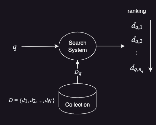
A ranking model $f(q, d)$ scores each document $d$ in a set $D$ based on its relevance to a query $q$. To formalize this, we can label the $n$ documents in $D$ with integers from ${1, 2, \cdots, n}$. A ranking list is a permutation $\pi$ on $D$, where $\pi(j)$ denotes the rank of the $j$-th document. Let $\Pi$ represent the set of all possible permutations. The goal of ranking is then to select the best permutation $\pi \in \Pi$ for a query $q$ based on the scores produced by $f(q, d)$.
For the ranking model $f(q,d)$, many approaches have been proposed in IR literature. In general, they can be categorzied into query-dependent models and query-independent models.
Query-dependent Models
Query-dependent models rank documents based on the similarity between the query and the content of the document. For this reason, they are often referred to as content-based models.
The most intuitive query-dependent model is the vector space model (VSM). In VSM, both documents and queries are represented as vectors in a Euclidean space. With this representation, the similarity between a document and a query can be measured by calculating the inner product of the two vectors.
Probabilistic models are more advanced and among the most widely used query-dependent models. These models rank documents based on the probability that a document is relevant to a given query. So, $f(d,q)=P(R=1 \vert d,q)$. The most famouse probabilistic models include BM25 and the language model for information retrieval (LMIR). See my previous posts for more details on BM25 and the LMIR.
While these traditional probabilistic models work well for many retrieval tasks, one limitation is that they lack a concept of document quality. Because they only consider how well a query matches a document, they ignore other potentially important signals, such as user clicks, recency, or spam indicators.
Query-independent Models
Query-independent models rank documents based on their own importance. Thus, these models are blind to the query.
Link-based ranking models are in this category. The most famous link-based model is PageRank. It measures the authority or importance of a webpage by considering the number and quality of hyperlinks pointing to the page. So, it has been widely used in web search. See my previous post for more details on PageRank.
However, query-independent models such as PageRank cannot evaluate topical relevance or context on their own. This leaves the possibility that a highly authoritative but completely irrelevant document may appear at the top of the search results.
Given that there is no single perfect ranking model, it is natural to expect that combining multiple signals into a ranking model would improve search systems.
Core Idea
The goal of learning to rank is to stop relying on a single ranking method. Instead, it uses machine learning to automatically construct a ranking model $f(q,d)$ that incorporates multiple signals.
For example, we can learn a ranking model $f(q,d)$ with two features: BM25 and PageRank. In this way, we can rank documents by leveraging both query-dependent and query-independent scores.
This ability to combine multiple features is a significant advantage of learning to rank for the following reasons:
- It makes it easy to incorporate advances in retrieval models simply by including the output of a new model as one feature.
- It makes the retrieval system more robust by making it harder for spammers to manipulate the ranking.
Learning-to-Rank Framework
Like a typical machine learning framework, a learning-to-rank framework has a specific input space and output space. Each space has the following structure:
- The input space $\mathcal{X}$ consists of lists of feature vectors. Thus, an element $x \in \mathcal{X}$ represents a single list of feature vectors.
- The output space $\mathcal{Y}$ consists of lists of relevance grades. Thus, an element $y \in \mathcal{Y}$ represents a single list of relevance grades.
Since learning to rank is a supervised learning task, the training data must be shaped to these input and output spaces.
Training Data and Data Labeling
The training data consists of $m$ training queries $q_i(i=1,\dots,m)$, where $q_i$ is the $i$-th query. The training queries can be selected from search log data, either randomly or based on their frequencies. Each query $q_i$ is then associated with a set of documents $D_i = {d_{i,1}, \dots, d_{i,n_i}}$ and the corresponding relevance judgments:
\[\mathbf{y}_i = \{y_{i,1}, \dots, y_{i,n_i}\}\]where $n_i$ is the size of $D_i$ and $\mathbf{y}_i$.
More specifically, $d_{i,j}$ is the $j$-th document in $D_i$, and $y_{i,j} \in Y$ is the relevance judgment of $d_{i,j}$ with respect to $q_i$.
For the target labels, we should define a list of grades, or levels. Suppose that we define a list of grades numbered from 1 to $l$, ranked from lowest to highest. A higher number means a better grade, so $l$ is the highest grade ($l \succ l - 1 \succ \cdots \succ 1$). This is the label set $Y = {1,2, \cdots, l}$. In practice, $l$ is often chosen to be between 4 and 5. For example, if $l=5$, then each grade can be interpreted as follows:
- 5: perfect
- 4: excellent
- 3: good
- 2: fair
- 1: bad
For data labeling, there are two main approaches:
- Human judgments
- Click-through log mining
In the human judgment approach, human assessors are asked to judge the relevance of each retrieved document using $l$ relevance levels. However, this approach is not very practical for large-scale search systems. From a machine learning point of view, a few hundred queries are usually not enough to train and evaluate a learning-to-rank algorithm reliably. Human labeling is also expensive and time-consuming, especially as the number of queries and documents grows.
In click-through log mining, search log data, such as click-through logs, is used. In this case, user interactions are used as implicit feedback. For example, if a user clicks a document after submitting a query, the clicked document can be treated as more relevant than the documents that were skipped. This approach is more scalable because search engines can collect large amounts of interaction data from real users. However, click data is noisy. A clicked document is not always relevant, and an unclicked document is not always irrelevant. Therefore, click-through data should be handled carefully when used for learning to rank. See my previous post for more details on relevance feedback.
We represent the original training data as:
\[S = \{(q_i, D_i), \mathbf{y}_i\}_{i=1}^m\]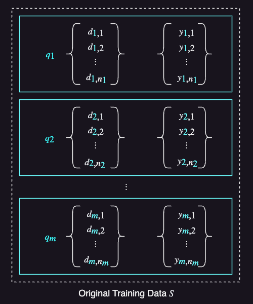
Below is just an illustrative example of the original training data in Python:
S = [
    # For q1:
    {"qid": 1, "query": "hello world", "doc": {...}, "relevance": 3},
    {"qid": 1, "query": "hello world", "doc": {...}, "relevance": 3},
    {"qid": 1, "query": "hello world", "doc": {...}, "relevance": 1},
    {"qid": 1, "query": "hello world", "doc": {...}, "relevance": 3},
    # For q2:
    {"qid": 2, "query": "chocolate milkshake", "doc": {...}, "relevance": 1},
    {"qid": 2, "query": "chocolate milkshake", "doc": {...}, "relevance": 1},
    {"qid": 2, "query": "chocolate milkshake", "doc": {...}, "relevance": 2},
    {"qid": 2, "query": "chocolate milkshake", "doc": {...}, "relevance": 3},
    {"qid": 2, "query": "chocolate milkshake", "doc": {...}, "relevance": 3},
]
Note that we also assign a qid to each row in the original training data.
We’ll discuss why this matters shortly.
The original training data contains raw objects such as queries, documents, and relevance judgments. For a machine learning algorithm to process the training data, these objects need to be represented as numbers. To do this, we extract feature vectors that reflect the relevance of documents to the query. A feature vector $x_{i,j} = \phi(q_i, d_{i,j})$ is created from each query-document pair $(q_i, d_{i,j})$, where $i = 1, 2, \cdots, m$ and $j = 1, 2, \cdots, n_i$, and $\phi$ is the feature extractor, or feature function.
Here is an example of a feature function that extracts two features: BM25 and PageRank scores:
def extract_features(query: str, document: dict) -> list[float]:
    """
    Extract features based on the query and document.
    """
    bm25_score = get_bm25_score(query, document)
    pagerank_score = get_pagerank_score(document)  # pagerank scores are scaled

    return [bm25_score, pagerank_score]
We represent the feature-based training data as:
\[S' = \{(x_i,y_i)\}^m_{i=1}\]where $x_i = {x_{i,1},x_{i,2},\cdots,x_{i,n_i}}$.
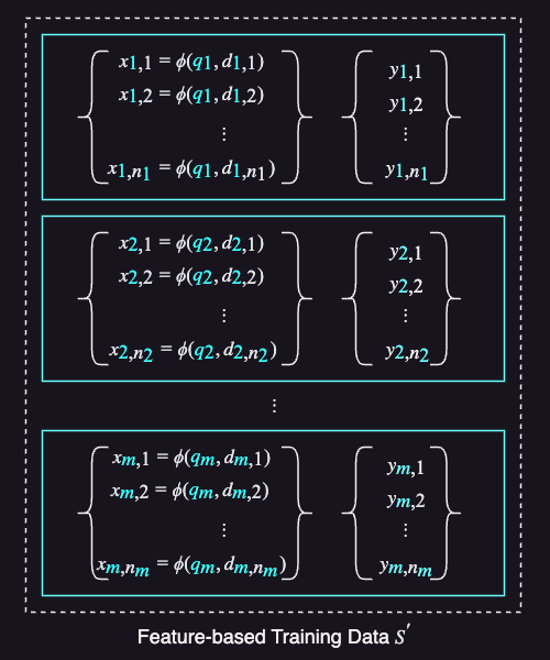
The following code uses the feature function to transform the original training data into a feature-based training data:
S_prime = []
for item in S:
    features = extract_features(item["query"], item["doc"])
    S_prime.append(
        {
            "qid": item["qid"],
            "features": features,
            "relevance": item["relevance"],
        }
    )
As a result, S_prime may look like this:
S_prime = [
    # For qid 1:
    {"qid": 1, "features": [11.9413, 115], "relevance": 3},
    {"qid": 1, "features": [21.8816, 126], "relevance": 3},
    {"qid": 1, "features": [17.145, 126], "relevance": 1},
    {"qid": 1, "features": [16.5712, 122], "relevance": 3},
    # For qid 2:
    {"qid": 2, "features": [1, 260], "relevance": 1},
    {"qid": 2, "features": [19.617, 240], "relevance": 1},
    {"qid": 2, "features": [24.358, 3052], "relevance": 2},
    {"qid": 2, "features": [44.9817, 4871], "relevance": 3},
    {"qid": 2, "features": [36.8917, 11208], "relevance": 3},
]
Here’s why we keep qid in the training data.
In learning to rank, each training instance corresponds to one query group, so all rows with the same qid should be kept together.
When splitting the data into training and test sets, we should split by query group not by individual rows.
For example, all rows with qid=1 should go into either the training set or the test set, but not both.
In practice, training data is often stored in a file so that it is easy to load, share and reuse. One common choice for learning-to-rank datasets is the LETOR (SVMLight) format. It is a text-based format that stores relevance labels, query IDs, and feature values. The structure is:
<relevance> qid:<query_id> <feature_id>:<value> ...
The following Python code saves the training data in our example (S_prime) in a LETOR file named train.txt:
def save_training_data(training_data: list[dict], output_path: str) -> None:
    """
    Save relevance labels, query IDs, and feature vectors in LETOR format.
    """
    with open(output_path, "w", encoding="utf-8") as file:
        for item in sorted(training_data, key=lambda row: row["qid"]):
            features = " ".join(
                f"{feature_id}:{value}"
                for feature_id, value in enumerate(item["features"], start=1)
            )
            file.write(f"{item['relevance']} qid:{item['qid']} {features}\n")


save_training_data(S_prime, "train.txt")
Output:
3 qid:1 1:11.9413 2:115
3 qid:1 1:21.8816 2:126
1 qid:1 1:17.145 2:126
3 qid:1 1:16.5712 2:122
1 qid:2 1:1 2:260
1 qid:2 1:19.617 2:240
2 qid:2 1:24.358 2:3052
3 qid:2 1:44.9817 2:4871
3 qid:2 1:36.8917 2:11208
Each row represents one query-document pair.
The first number is the relevance grade, qid:1 identifies the query group, and the remaining entries contain feature IDs and values.
Here, feature 1 is the BM25 score, and feature 2 is the PageRank score.
Evaluation and Loss Function
The performance of a ranking model can be evaluated by comparing the ranked lists produced by the model with the ground-truth relevance labels. Common evaluation metrics used in IR are MAP(Mean Average Precision), DCG (Discounted Cumulative Gain), and NDCG(Normalized Discounted Cumulative Gain). We take NDCG as an example because it’s the de facto standard evaluation metric in learning to rank.
Let’s first look at DCG. DCG measures the quality of a ranked list by summing the relevance gains of the top $k$ documents. It gives higher weight to documents near the top because users are more likely to look at earlier results.
DCG@k is defined as:
\[DCG@k = \sum_{j=1}^{k} \frac{G_j}{\log_2(j + 1)}\]where $G_j(\cdot)$ is a gain function and $\log_2(j + 1)$ is the position discount. A common choice of gain is $G_j = 2^{rel_j} - 1$, where $rel_j$ is the relevance grade of the document at rank $j$. This means highly relevant documents get more reward when they appear earlier. However, raw DCG scores are hard to compare across queries because each query can have a different number of relevant documents.
NDCG normalizes the metric to a $[0, 1]$ scale for consistent evaluation across queries:
\[NDCG@k = \frac{DCG@k}{IDCG@k}\]where $IDCG(k)$ (Ideal DCG) is the maximum possible DCG at position $k$. This peak score is achieved by a perfect ranking, where documents are sorted in descending order of their relevance grades. Because of this, NDCG rewards models that rank highly relevant documents near the top. As a result, for a perfect ranking, the NDCG score is $1$. See my previous post for more details on DCG and NDCG.
We can formalize this idea as follows. Suppose a ranking model produces a ranked list $F(\mathbf{x})$ for a query, and the ground-truth relevance labels are given by $\mathbf{y}$. We can define a loss function based on NDCG as follows:
\[L(F(\mathbf{x}), \mathbf{y}) = 1.0 - NDCG\]Here, NDCG measures how good the predicted ranking is compared with the ideal ranking. If the model produces a perfect ranking, then $NDCG = 1.0$, so the loss becomes 0. Therefore, learning to rank can be viewed as learning a ranking function that minimizes this evaluation loss.
Approaches
Learning-to-rank algorithms are generally categorized into three approaches:
- pointwise approach
- pairwise approach
- listwise approach
Each approach models the ranking problem differently. They use different input and output spaces, hypotheses, and loss functions. Even with the same relevance judgments, different approaches can derive different ground-truth labels for learning.
Pointwise Approach
In the pointwise approach, ranking is treated as a standard supervised learning problem, such as classification, regression, or ordinal classification. Each query-document pair is considered independently, and the model predicts the relevance score of each document.
In this setting:
- The input space $\mathcal{X}$ contains the feature vector of each individual document.
- The output space $\mathcal{Y}$ contains the relevance degree of each individual document.
- The loss function $L(\cdot)$ measures how accurately the model predicts the ground-truth label for each individual document.
In practice, the ranking process is as follows:
- For each query-document pair $(q_i, d_{i,j})$, extract a feature vector $x_{i,j}$.
- Use the trained model $f(x)$ to predict a relevance score $\hat{y}_{i,j}$ for each document independently.
- Sort the documents for the same query by their predicted relevance scores.
- Return the sorted list as the final ranking.
An important limitation of this approach is that the group structure of ranking is ignored. This is because it does not consider the interdependence among documents in the same ranked list. In other words, it ignores the fact that multiple documents are associated with the same query. As a result, the loss function is unaware of each document’s position in the final ranking. This is a limitation because common IR evaluation measures, such as MAP and NDCG, are query-level and position-based.
Some pointwise approaches include:
- SLR (Staged Logistic Regression) (1992)
- PRanking (2001)
- McRank (2007)
Pairwise Approach
In pairwise approach, pairs of documents are ranked into a relative order.
In this setting:
- The input space $\mathcal{X}$ contains pairs of documents, where each document is represented as a feature vector.
- The output space $\mathcal{Y}$ contains the pairwise preference between two documents, usually represented by values such as ${1, -1}$.
- The loss function $L(\cdot)$ measures the inconsistency between the predicted preference and the ground-truth label.
In practice, the ranking process is as follows:
- For each query, construct pairs of documents from the retrieved document set.
- For each document pair $(d_u, d_v)$, extract their feature vectors $x_u$ and $x_v$.
- Use the trained model $f(x)$ to predict which document in each pair should be ranked higher.
- Combine the pairwise preferences to produce a final ranked list.
- Return the sorted list as the final ranking.
Considering that the loss function used in the pairwise approach only considers the relative order between two documents, the pairwise approach has the same limitation as the pointwise approach. That is, it also ignores the group structure of ranking.
Some pairwise approaches include:
- Ranking SVM (2000)
- RankBoost (2003)
- RankNet (2005)
Listwise Approach
In the listwise approach, an entire list of documents is ordered at once.
In this setting:
- The input space $\mathcal{X}$ contains the entire group of documents for a query, where each document is represented as a feature vector.
- The output space $\mathcal{Y}$ contains either a ranked list (permutation) of the documents, or the relevance degrees of all documents associated with the query.
- The loss function $L(\cdot)$ either measures the difference between the predicted ranked list and the ground-truth ranked list (when the output space contains a permutation), or approximates IR evaluation measures (when the output space contains the relevance degrees).
In practice, the ranking process is as follows:
- For each query, collect the list of retrieved documents.
- Extract a feature vector for each document in the list.
- Use the trained model $f(x)$ to score or directly order the entire document list.
- Return the ordered list as the final ranking.
Unlike the pointwise and pairwise approaches, the listwise approach preserves the group structure of ranking. It also allows ranking evaluation measures like NDCG to be incorporated more directly into the loss function during learning.
In practice, listwise approaches often perform better than pairwise and pointwise approaches. A large scale experiment comparing different learning-to-rank methods support this statement (source).
Some listwise approaches include:
- ListNet (2007)
- ListMLE (2008)
- LambdaMART (2010)
We take LambdaMART as an example.
LambdaMART with LightGBM
LambdaMART is one of the most popular learning-to-rank algorithms used today, thanks to its strong empirical performance with low inference latency. It combines LambdaRank, which is designed for optimizing ranking quality, with MART, a gradient-boosted decision tree method.
LambdaMART is often categorized as both a pairwise and listwise approach. It is considered pairwise because it uses pairwise preferences between documents during training. At the same time, it is also considered listwise because those pairwise updates are guided by a ranking metric such as NDCG, which evaluates the quality of the entire ranked list. Because of this, LambdaMART can be viewed as a hybrid approach that connects pairwise learning with listwise ranking objectives.
LightGBM is a gradient boosting framework developed by Microsoft.
It is widely used for tabular machine learning tasks due to its speed and scalability in practice.
For learning-to-rank tasks, LightGBM provides LGBMRanker, which supports ranking objectives such as lambdarank.
Thanks to this, training a LambdaMART ranking model with Python is simple and straightforward.
Refer to the LightGBM’s installation guide to install lightgbm in your environment.
The code examples below were tested with LightGBM 4.7.0.
Also install scikit-learn for loading the dataset:
pip install scikit-learn
For our experimentation, we’ll use Microsoft’s MSLR-WEB10K dataset. It’s a widely used public LETOR dataset for learning to rank. It contains 10,000 queries, with 136 extracted features for each query-document pair. So we don’t need the feature extractor for this demonstration. Its relevance judgments range from 0 (irrelevant) to 4 (perfectly relevant). So, its label set is $Y = {0,1,2,3,4}$.
The features cover both query-dependent and query-independent signals, including the familiar BM25 and PageRank signals. For example:
| Feature ID | Description |
|---|---|
| 106–110 | BM25 for body, anchor, title, URL, and whole document. |
| 111–125 | LMIR scores with different smoothing methods. |
| 130 | PageRank. |
| 134–136 | Click and dwell-time signals. |
Microsoft provides five folds, each with separate train.txt, test.txt, and vali.txt files split by query.
We’ll use the train.txt and test.txt in the first fold (Fold1), keeping their existing split.
Here’s how to use LigtGBM’s LGBMRanker to train a LambdaMART ranking model:
import lightgbm as lgb
import numpy as np
from scipy.sparse import csr_matrix
from sklearn.datasets import load_svmlight_file

N_FEATURES: int = 136  # Number of features in the MSLR-WEB10K dataset


def _load_letor_data(file_path: str) -> tuple[csr_matrix, np.ndarray, np.ndarray]:
    """
    Load feature vectors, relevance labels, and query IDs from a LETOR file.
    """
    X, y, qids = load_svmlight_file(
        file_path,
        n_features=N_FEATURES,
        query_id=True,  # keeps query IDs separate from the features
        zero_based=False,  # LETOR files are 1-based indexed
        dtype=np.float32,
    )
    X.eliminate_zeros()  # Remove explicit zeros to save memory
    return X, y.astype(np.int32), qids


def _group_by_query(
    X: csr_matrix, y: np.ndarray, qids: np.ndarray
) -> tuple[csr_matrix, np.ndarray, np.ndarray]:
    """
    Sort rows by query ID and calculate the number of documents per query.
    """
    order = np.argsort(qids, kind="stable")
    _, groups = np.unique(qids[order], return_counts=True)
    return X[order], y[order], groups


def train_model(training_file: str, test_file: str, random_state: int = 42) -> lgb.LGBMRanker:
    """
    Train a LightGBM ranking model using LambdaMART.

    Args:
        training_file: Path to the supplied train.txt file.
        test_file: Path to the supplied test.txt file from the same fold.
        random_state: Random seed for reproducibility.

    Returns:
        Trained LGBMRanker model.
    """
    # Load the training and test data from LETOR files
    X_train, y_train, qids_train = _load_letor_data(training_file)
    X_test, y_test, qids_test = _load_letor_data(test_file)
    assert np.intersect1d(qids_train, qids_test).size == 0, "Query overlap between splits"

    # Sort by qid to ensure proper grouping
    X_train, y_train, group_train = _group_by_query(X_train, y_train, qids_train)
    X_test, y_test, group_test = _group_by_query(X_test, y_test, qids_test)
    print(f"Training set: {len(group_train)} queries, {X_train.shape[0]} query-document pairs")
    print(f"Test set: {len(group_test)} queries, {X_test.shape[0]} query-document pairs")
    print(f"Features: {X_train.shape[1]}")

    # Initialize and train the LightGBM ranking model
    model = lgb.LGBMRanker(
        objective="lambdarank",
        metric="ndcg",
        n_estimators=100,
        random_state=random_state,
        n_jobs=4,
    )
    model.fit(
        X_train,
        y_train,
        group=group_train,
        eval_set=[(X_test, y_test)],
        eval_group=[group_test],
        eval_metric="ndcg",
        eval_at=[5, 10],
    )

    print("Feature importances (top 10 by split count):")
    importances = model.feature_importances_
    for column in np.argsort(-importances, kind="stable")[:10]:
        print(f"  Feature {column + 1}: {importances[column]}")

    print("Evaluation results:")
    for metric, values in model.evals_result_["valid_0"].items():
        print(f"  {metric}: {values[-1]:.4f}")

    return model


training_file: str = "train.txt"
test_file: str = "test.txt"
model = train_model(training_file, test_file)
This code first loads the LETOR-style training and test data using scikit-learn’s load_svmlight_file.
Next, _group_by_query sorts each split by query ID and calculates the number of documents for each query.
This is because learning-to-rank models learn from groups of documents associated with the same query.
If we split the data by individual rows, documents from the same query could appear in both the training and test sets.
This would make the evaluation less reliable.
The group sizes are passed to LightGBM through the group and eval_group arguments.
This tells LGBMRanker which consecutive rows belong to the same query group.
For example, group=[10, 20] means that the first 10 rows belong to one query and the next 20 to another.
Finally, the model is trained and evaluated with NDCG at positions 5 and 10 through the eval_at argument.
In this code, the model’s objective parameter is specified as lambdarank.
This tells LightGBM to train a gradient-boosted ranking model using the LambdaRank-style ranking objective.
Together, gradient-boosted decision trees and the LambdaRank objective correspond to the LambdaMART approach.
The model trains for a fixed 100 iterations (n_estimators), and the code reports the final test scores.
To tune the model, you should use the vali.txt instead of selecting settings based on the test results.
For more information about LGBMRanker, refer to the documentation.
When you run this example, you’ll see the following output:
Training set: 6000 queries, 723412 query-document pairs
Test set: 2000 queries, 241521 query-document pairs
Features: 136
Feature importances (top 10 by split count):
  Feature 130: 143
  Feature 133: 130
  Feature 127: 119
  Feature 129: 117
  Feature 131: 102
  Feature 108: 97
  Feature 126: 90
  Feature 135: 87
  Feature 14: 86
  Feature 15: 82
Evaluation results:
  ndcg@5: 0.4850
  ndcg@10: 0.5032
Feature importances show how often each feature was used in the model’s tree splits. A higher importance value means that the feature was used in more splits. If we plot the feature importances with the corresponding feature names from the documentation, we get:
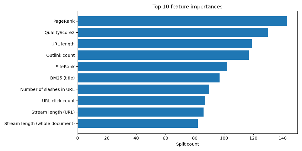
The evaluation results show how well the trained model performs on the test set. Higher NDCG values indicate better ranking performance.
In practice, we save the trained model to a file so that it can be loaded later and used to rank documents without retraining. To do so:
import os

...


def save_model(model: lgb.LGBMRanker, output_path: str) -> str:
    """
    Save the trained model to a file.

    Args:
        model: The trained LGBMRanker model.
        output_path: Path to save the model.

    Returns the path to the saved model.
    """
    output_dir = os.path.dirname(os.path.abspath(__file__))
    output_path = os.path.join(output_dir, output_path)
    model.booster_.save_model(output_path)
    print(f"Model saved to {output_path}")

    return output_path


training_file: str = "train.txt"
test_file: str = "test.txt"
model = train_model(training_file, test_file)
save_model(model, "ltr_model.txt")
Now that we’ve saved our ranking model as ltr_model.txt, let’s use it to rank documents.
Ranking Scheme
Using a machine learning model to rank hundreds or thousands of documents can be computationally expensive and slow. Besides, users typically expect search results to be returned within a few hundred milliseconds. For this reason, applying a complex ranking model to every document in the collection is impractical, especially when the system needs to handle a large volume of search requests. A common solution is to use a two-phase ranking scheme, also known as a multi-stage retrieval pipeline.
In a two-phase scheme, retrieval is done as follows:
- In the first phase, a cheap and fast retrieval model, such as BM25, is used to retrieve a small number of potentially relevant documents (or candidates). This phase is also called top-$k$ document retrieval.
- In the second phase, a more computationally expensive but more accurate machine-learned model is used to the smaller set of documents retrieved in the first phase. This phase is also called re-ranking.
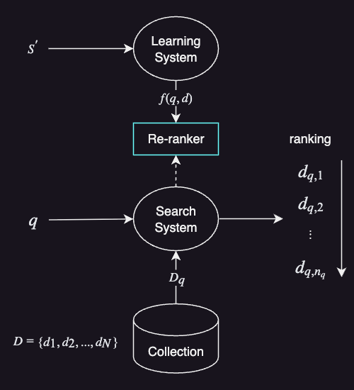
Let’s continue with our example to illustrate this process.
We’ll use the documents associated with the first query in test.txt as our ranking candidates:
X_test, y_test, qids_test = _load_letor_data(test_file)

# Get the first query ID from the test set.
query_id = int(qids_test[0])

# Find the indices of all documents belong to the first query.
rows = np.flatnonzero(qids_test == query_id)

# Extract the features of the candidate documents for the first query.
candidate_features = X_test[rows]
We’ll assume that candidate_features are the features of documents retrieved in the first phase.
In real-world applications, we would use a feature extractor to get the features for each candidate document before re-ranking.
To load the trained model from the file ltr_model.txt, we’ll use:
def load_model(model_path: str) -> lgb.Booster:
    """
    Load a trained LightGBM model from a file.
    """
    model = lgb.Booster(model_file=model_path)
    print(f"Model loaded from {model_path}")
    return model
The following function predicts relevance scores from the given features, and sort them in descending order:
def rerank(model: lgb.LGBMRanker | lgb.Booster, features: csr_matrix) -> list[dict]:
    """
    Re-rank candidate documents using their precomputed features.
    """
    # Predict scores
    scores = model.predict(features)

    # Attach scores and sort candidates by predicted score in descending order
    reranked = sorted(
        ({"candidate_index": index, "score": float(score)} for index, score in enumerate(scores)),
        key=lambda doc: doc["score"],
        reverse=True,
    )

    return reranked
We can then rerank the candidates and print the top 10 results:
model = load_model("ltr_model.txt")
ranked_results = rerank(model=model, features=candidate_features)
print(f"Top 10 documents for test query {query_id}:")
for doc in ranked_results[:10]:
    index = int(rows[doc["candidate_index"]])
    print(f"Row: {index + 1}, Relevance: {int(y_test[index])}, Score: {doc['score']:.4f}")
The output is:
Model loaded from ltr_model.txt
Top 10 documents for test query 13:
Row: 89, Relevance: 2, Score: 1.6108
Row: 87, Relevance: 3, Score: 1.1052
Row: 56, Relevance: 2, Score: 1.0883
Row: 77, Relevance: 3, Score: 1.0858
Row: 48, Relevance: 0, Score: 0.9859
Row: 115, Relevance: 2, Score: 0.9353
Row: 64, Relevance: 1, Score: 0.9299
Row: 35, Relevance: 1, Score: 0.8826
Row: 59, Relevance: 1, Score: 0.8621
Row: 114, Relevance: 1, Score: 0.8517
The candidates are ranked by their predicted Score, from highest to lowest.
Here, Row refers to the document’s row number in test.txt.
The relevane scores are just shown for comparison.
We can see that higher-ranked documents generally have higher relevance labels than lower-ranked ones.
Note that the predicted scores are relative ranking scores and do not represent absolute relevance.
Conclusion
Learning to rank has been studied extensively since the 2000s. Many of the foundational ideas developed during that period are still widely used today.
With advances in machine learning, especially the rise of LLMs, we now have more options for building search systems. Modern search systems often combine traditional learning-to-rank methods with neural retrievers and cross-encoder rerankers. LLM-based rerankers are also becoming an interesting option.
These newer approaches aren’t necessarily replacing traditional methods. Instead, they’re giving us more ways to build better search systems, each with its own trade-offs in ranking quality, speed, and cost.
References
- A Short Introduction to Learning to Rank by Hang Li
- Learning to Rank for Information Retrieval by Tie-Yan Liu
- Learning to rank - Wikipedia
- Microsoft Learning to Rank Datasets